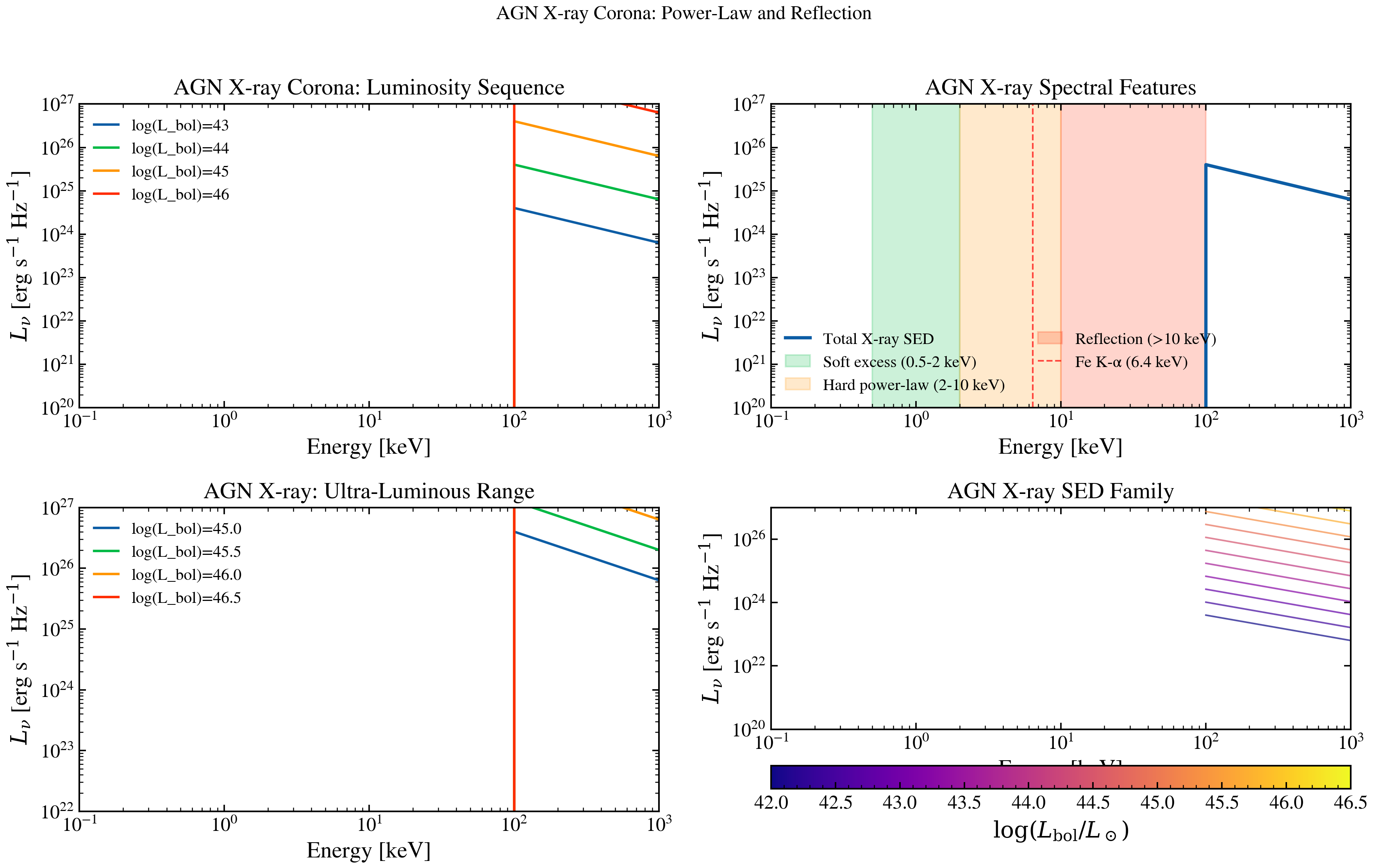
AGN X-ray Emission and Corona

Plot the X-ray spectrum from AGN coronae showing power-law continuum, reflection hump, and iron K-alpha line. Demonstrates how the X-ray spectrum depends on AGN bolometric luminosity and accretion efficiency.

import jax.numpy as jnp
import matplotlib.pyplot as plt
import numpy as np

from tengri.analysis.plotting import setup_style
from tengri.xray import xray_agn_corona

setup_style()

# Wavelength grid spans 0.1 keV (124 A, the function's soft cutoff) up to 1000 keV
# (0.0124 A). The xray_agn_corona function zeros output for lambda > 124 A.
# Conversion: E[keV] = 12398 / lambda[A].
wavelength = jnp.logspace(np.log10(0.0124), np.log10(124.0), 512)  # Angstrom
# E[keV] = hc/lambda with hc = 12.398 keV*A, so E[keV] = 12.398 / lambda[A].
wave_keV = 12.398 / np.array(wavelength)

fig, axes = plt.subplots(2, 2, figsize=(12, 8))

# --- Panel 1: Luminosity dependence ---
ax = axes[0, 0]

for log_lbol in [43.0, 44.0, 45.0, 46.0]:
    L_bol = 10.0**log_lbol  # erg/s
    l_xray = xray_agn_corona(wavelength, L_agn_bol=L_bol)
    ax.loglog(wave_keV, np.array(l_xray), lw=1.5, label=f"log(L_bol)={log_lbol:.0f}")

ax.set_xlabel("Energy [keV]")
ax.set_ylabel(r"$L_\nu$ [erg s$^{-1}$ Hz$^{-1}$]")
ax.set_title("AGN X-ray Corona: Luminosity Sequence")
ax.legend(fontsize=10, frameon=False)
ax.set_xlim(0.1, 1000)
ax.set_ylim(1e22, 1e27)

# --- Panel 2: Show X-ray continuum shape (Compton reflection) ---
ax = axes[0, 1]

log_lbol = 44.0
L_bol = 10.0**log_lbol

l_xray = xray_agn_corona(wavelength, L_agn_bol=L_bol)

# Highlight key X-ray features
ax.loglog(wave_keV, np.array(l_xray), "C0-", lw=2.0, label="Total X-ray SED")

# Annotate key features
# Soft X-ray bump (0.5-2 keV)
ax.axvspan(0.5, 2.0, alpha=0.2, color="C1", label="Soft excess (0.5-2 keV)")
# Hard X-ray power-law (2-10 keV)
ax.axvspan(2.0, 10.0, alpha=0.2, color="C2", label="Hard power-law (2-10 keV)")
# Reflection hump (10-100 keV)
ax.axvspan(10.0, 100.0, alpha=0.2, color="C3", label="Reflection (>10 keV)")
# Iron K-alpha line
ax.axvline(6.4, color="red", ls="--", lw=1.0, alpha=0.7, label="Fe K-α (6.4 keV)")

ax.set_xlabel("Energy [keV]")
ax.set_ylabel(r"$L_\nu$ [erg s$^{-1}$ Hz$^{-1}$]")
ax.set_title("AGN X-ray Spectral Features")
ax.legend(fontsize=10, frameon=False, ncol=2)
ax.set_xlim(0.1, 1000)
ax.set_ylim(1e22, 1e27)

# --- Panel 3: High-luminosity AGN ---
ax = axes[1, 0]

for log_lbol in [45.0, 45.5, 46.0, 46.5]:
    L_bol = 10.0**log_lbol
    l_xray = xray_agn_corona(wavelength, L_agn_bol=L_bol)
    ax.loglog(wave_keV, np.array(l_xray), lw=1.5, label=f"log(L_bol)={log_lbol:.1f}")

ax.set_xlabel("Energy [keV]")
ax.set_ylabel(r"$L_\nu$ [erg s$^{-1}$ Hz$^{-1}$]")
ax.set_title("AGN X-ray: Ultra-Luminous Range")
ax.legend(fontsize=10, frameon=False)
ax.set_xlim(0.1, 1000)
ax.set_ylim(1e22, 1e27)

# --- Panel 4: Spectral index vs luminosity (implicit) ---
ax = axes[1, 1]

log_lbol_range = np.linspace(42.0, 46.5, 12)
colors = plt.cm.plasma(np.linspace(0, 1, len(log_lbol_range)))

for log_lbol, color in zip(log_lbol_range, colors):
    L_bol = 10.0**log_lbol
    l_xray = xray_agn_corona(wavelength, L_agn_bol=L_bol)
    mask = np.array(l_xray) > 0
    ax.loglog(wave_keV[mask], np.array(l_xray)[mask], lw=1.0, color=color, alpha=0.7)

ax.set_xlabel("Energy [keV]")
ax.set_ylabel(r"$L_\nu$ [erg s$^{-1}$ Hz$^{-1}$]")
ax.set_title("AGN X-ray SED Family")
ax.set_xlim(0.1, 1000)
ax.set_ylim(1e22, 1e27)

# Colorbar-like legend
sm = plt.cm.ScalarMappable(
    cmap=plt.cm.plasma, norm=plt.Normalize(vmin=log_lbol_range.min(), vmax=log_lbol_range.max())
)
sm.set_array([])
cbar = fig.colorbar(sm, ax=ax, orientation="horizontal", pad=0.12, aspect=25)
cbar.set_label(r"$\log(L_{\mathrm{bol}} / L_\odot)$")

fig.suptitle("AGN X-ray Corona: Power-Law and Reflection", fontsize=12)
fig.tight_layout(rect=[0, 0.04, 1, 0.97])
plt.savefig("plot_xray_agn.png", dpi=150, bbox_inches="tight")
plt.show()