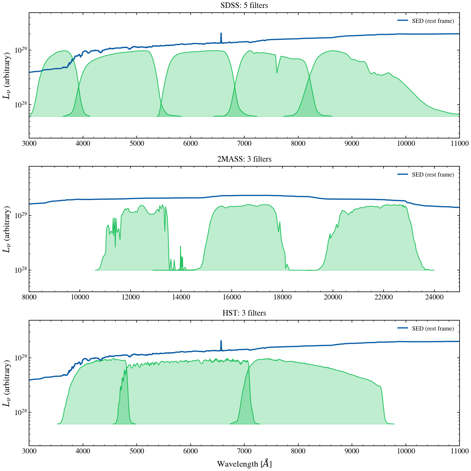
Filter Set Comparison

Compare filter coverage from three different photometric surveys on the same mock galaxy SED — SDSS (optical ugriz), 2MASS (NIR JHKs), and HST (UV/optical ACS). Demonstrates how filter placement controls which spectral features are captured. Each panel overlays the filter throughputs (orange) on the same underlying SED (blue).

from pathlib import Path

import matplotlib.pyplot as plt
import numpy as np

from tengri import (
    Fixed,
    Observation,
    Parameters,
    Photometry,
    SEDModel,
    load_filter_set,
    load_ssp_data,
)
from tengri.analysis.plotting import setup_style

setup_style()


def _find_ssp():
    """Locate SSP data from project root or docs/ (sphinx-gallery) cwd."""
    name = "ssp_prsc_miles_chabrier_wNE_logGasU-3.0_logGasZ0.0.h5"
    for p in [
        Path("data") / name,
        Path("../data") / name,
        Path("../../data") / name,
        Path("../../../data") / name,
    ]:
        if p.exists():
            return str(p)
    return None


SSP_PATH = _find_ssp()
_FILTER_DIR = next(
    (
        str(d)
        for d in [
            Path("data/filters"),
            Path("../data/filters"),
            Path("../../data/filters"),
            Path("../../../data/filters"),
        ]
        if d.exists()
    ),
    "data/filters",
)
if SSP_PATH is None:
    raise FileNotFoundError("SSP data not found — skipping example")

# --- Setup ---
ssp_data = load_ssp_data(SSP_PATH)

# Three filter sets — chosen so all bands fit on the same UV-NIR axis.
filter_sets = {
    "SDSS": ["sdss_u", "sdss_g", "sdss_r", "sdss_i", "sdss_z"],
    "2MASS": ["2mass_j", "2mass_h", "2mass_ks"],
    "HST": ["hst_f435w", "hst_f606w", "hst_f814w"],
}

# Build common model (fixed parameters)
spec = Parameters(
    sfh_tsnorm_log_peak_sfr=Fixed(1.0),
    sfh_tsnorm_peak_lbt_gyr=Fixed(2.0),
    sfh_tsnorm_width_gyr=Fixed(1.5),
    sfh_tsnorm_skew=Fixed(0.3),
    sfh_tsnorm_trunc=Fixed(3.0),
    met_logzsol=Fixed(-0.2),
    dust_tau_bc=Fixed(0.4),
    dust_tau_diff=Fixed(0.2),
    dust_slope=Fixed(-0.7),
    redshift=Fixed(0.05),
)

# --- Plot three panels ---
# Larger figsize + per-panel xlim keeps each survey's bands centred and
# avoids tight_layout title/axis collisions on cramped 3-stack figures.
fig, axes = plt.subplots(3, 1, figsize=(11, 11))

# Per-survey wavelength windows (Angstrom) — chosen to frame the bands with
# breathing room either side instead of one shared 3000-25000 axis that
# squeezes the SDSS panel and shows mostly empty space for HST.
panel_xlim = {
    "SDSS": (3000, 11000),
    "2MASS": (8000, 25000),
    "HST": (3000, 11000),
}

# Median-smooth the SED for display so Hα/Hβ/[OIII] spikes don't overpower
# the continuum once we use log-y. The smoothed curve is for visualisation
# only; predicted broadband fluxes still use the spiky SED internally.
from scipy.ndimage import median_filter

for ax, (survey_name, bands) in zip(axes, filter_sets.items()):
    obs = Observation(
        photometry=Photometry.from_names(bands, cache_dir=_FILTER_DIR),
    )
    model = SEDModel(spec, ssp_data, observation=obs)

    pred = model.predict_rest_sed({})
    wave = np.asarray(pred.wavelength)
    sed = np.asarray(pred.sed)
    sed_smooth = median_filter(sed, size=51)

    waves, trans, curves = load_filter_set(bands, cache_dir=_FILTER_DIR)

    # SED line — smoothed continuum so emission lines don't dominate the eye.
    ax.semilogy(wave, sed_smooth, color="C0", lw=2.0, label="SED (rest frame)")

    # Filter throughputs: shaded band scaled to a fixed fraction of the
    # panel's continuum level so each filter is clearly visible above zero
    # on a log axis (filling from 0 doesn't render on log-y).
    xlo, xhi = panel_xlim[survey_name]
    panel_mask = (wave >= xlo) & (wave <= xhi)
    sed_continuum = np.median(sed_smooth[panel_mask])
    y_floor = sed_continuum * 0.05
    y_ceil = sed_continuum * 0.8
    for fc in curves:
        wave_f = np.array(fc.wave)
        trans_f = np.array(fc.trans) / np.max(fc.trans)
        scaled = y_floor + trans_f * (y_ceil - y_floor)
        ax.fill_between(wave_f, y_floor, scaled, alpha=0.25, color="C1")
        ax.plot(wave_f, scaled, lw=1.2, color="C1", alpha=0.8)

    ax.set_ylabel(r"$L_\nu$ (arbitrary)")
    ax.set_xlim(*panel_xlim[survey_name])
    ax.set_ylim(sed_continuum * 0.02, sed_continuum * 4)
    ax.set_title(f"{survey_name}: {len(bands)} filters", fontsize=13, pad=8)
    ax.legend(frameon=False, loc="upper right", fontsize=10)

axes[-1].set_xlabel(r"Wavelength [$\AA$]")
fig.tight_layout()
plt.savefig("plot_filter_set_comparison.png", dpi=150, bbox_inches="tight")
plt.show()