IGM Transmission Model Comparison

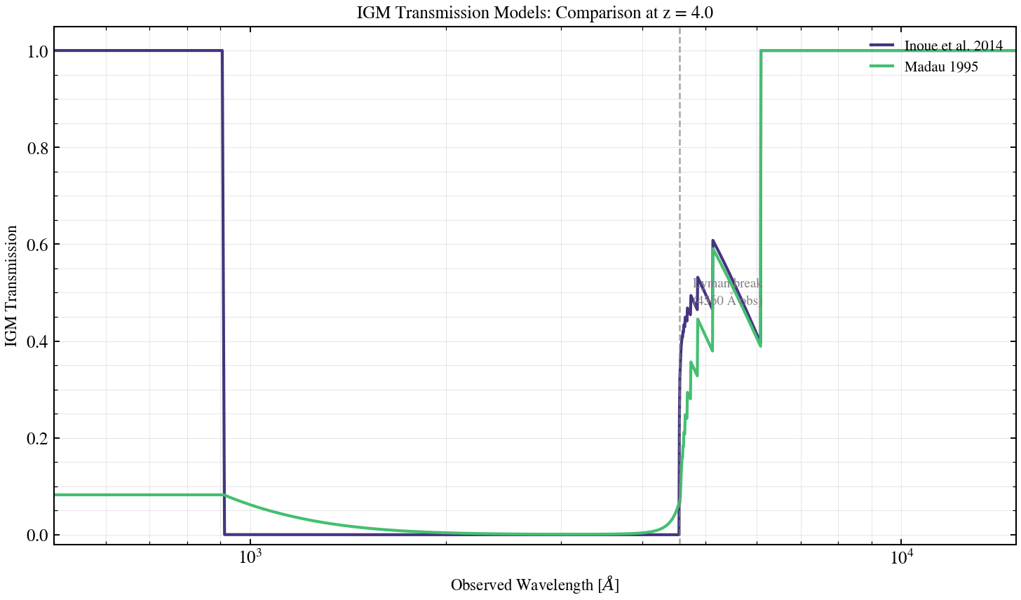
Compare available IGM transmission models at a fixed redshift (z=4.0). The Inoue et al. (2014) model captures Lyman-series absorption and Lyman-continuum opacity; the Madau (1995) model provides a simpler analytical approximation. This script shows how they differ in the UV to optical regime.

import jax
import jax.numpy as jnp
import matplotlib.pyplot as plt
import numpy as np

jax.config.update("jax_enable_x64", True)

from tengri.analysis.plotting import setup_style
from tengri.components.igm import (
    igm_transmission,
    igm_transmission_madau,
)

setup_style()

# Observed-frame wavelength grid covering Lyman break to optical
wave_obs = jnp.linspace(500.0, 15000.0, 2000)

# Fixed redshift for comparison
z_fixed = 4.0

fig, ax = plt.subplots(figsize=(10, 6))

# Inoue et al. 2014 model (default)
trans_inoue = np.array(igm_transmission(wave_obs, z_fixed))
ax.plot(
    np.array(wave_obs),
    trans_inoue,
    lw=2.0,
    color=plt.cm.viridis(0.15),
    label="Inoue et al. 2014",
)

# Madau 1995 model
trans_madau = np.array(igm_transmission_madau(wave_obs, z_fixed))
ax.plot(
    np.array(wave_obs),
    trans_madau,
    lw=2.0,
    color=plt.cm.viridis(0.70),
    label="Madau 1995",
)

# Mark Lyman break at 912 Å rest-frame
lyman_break_obs = 912.0 * (1 + z_fixed)
ax.axvline(lyman_break_obs, color="0.5", lw=1.2, ls="--", alpha=0.7)
ax.text(
    lyman_break_obs * 1.05,
    0.5,
    f"Lyman break\n({lyman_break_obs:.0f} Å obs)",
    fontsize=9,
    color="0.5",
    va="center",
)

ax.set_xlabel(r"Observed Wavelength [$\AA$]", fontsize=11)
ax.set_ylabel("IGM Transmission", fontsize=11)
ax.set_title(f"IGM Transmission Models: Comparison at z = {z_fixed}", fontsize=12)
ax.set_xscale("log")
ax.set_xlim(500, 15000)
ax.set_ylim(-0.02, 1.05)
ax.legend(fontsize=10, frameon=False, loc="upper right")
ax.grid(True, alpha=0.3, which="both")

fig.tight_layout()
plt.savefig("plot_igm_model_comparison.png", dpi=150, bbox_inches="tight")
plt.show()