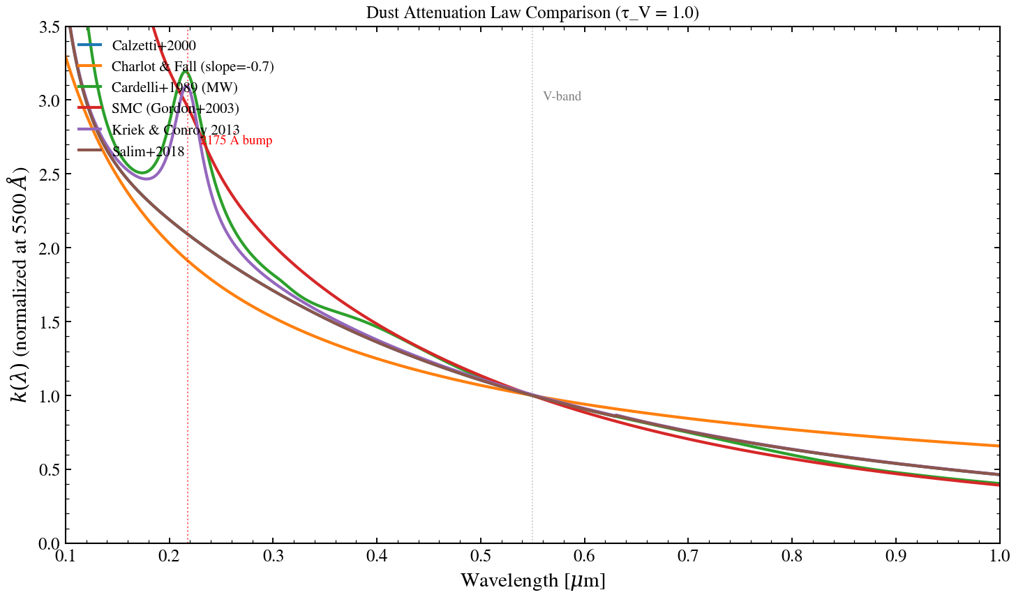
Attenuation Law Comparison

All major attenuation laws implemented in tengri evaluated at fixed τ_V = 1.0. Shows wavelength dependence (k(λ)) from UV through near-infrared, highlighting the UV bump (2175 Å) and the steepness differences between Milky Way, SMC, and starburst models.

import jax.numpy as jnp
import matplotlib.pyplot as plt
import numpy as np

from tengri.analysis.plotting import setup_style
from tengri.dust import resolve_dust_law

setup_style()

wavelength = jnp.linspace(1000.0, 10000.0, 2000)
wave_um = np.array(wavelength) / 1e4

# --- All major attenuation laws at τ_V = 1.0 ---
curves = [
    ("calzetti", {}, "Calzetti+2000"),
    ("power_law", {"n_slope": -0.7}, "Charlot & Fall (slope=-0.7)"),
    ("cardelli", {"dust_Rv": 3.1}, "Cardelli+1989 (MW)"),
    ("smc", {}, "SMC (Gordon+2003)"),
    ("kriek_conroy", {"dust_bump_strength": 1.0, "dust_delta": 0.0}, "Kriek & Conroy 2013"),
    ("salim", {}, "Salim+2018"),
]

# Use Tab10 for categorical colors (distinct, accessible)
colors = [
    "#1f77b4",  # blue
    "#ff7f0e",  # orange
    "#2ca02c",  # green
    "#d62728",  # red
    "#9467bd",  # purple
    "#8c564b",  # brown
]

fig, ax = plt.subplots(figsize=(10, 6))

for (name, kwargs, label), color in zip(curves, colors):
    dust_fn = resolve_dust_law(name)
    k = dust_fn(wavelength, **kwargs)
    ax.plot(wave_um, np.array(k), label=label, color=color, lw=2.0)

# --- Annotations ---
ax.axvline(0.55, ls=":", color="grey", lw=0.8, alpha=0.5)
ax.text(0.56, 3.0, "V-band", fontsize=9, color="grey")

ax.axvline(0.2175, ls=":", color="red", lw=1.0, alpha=0.6)
ax.text(0.23, 2.7, "2175 Å bump", fontsize=9, color="red")

ax.set_xlabel(r"Wavelength [$\mu$m]")
ax.set_ylabel(r"$k(\lambda)$ (normalized at 5500 $\AA$)")
ax.set_title("Dust Attenuation Law Comparison (τ_V = 1.0)", fontsize=12)
ax.set_xlim(0.1, 1.0)
ax.set_ylim(0, 3.5)
ax.legend(fontsize=10, frameon=False, loc="upper left", ncol=1)
fig.tight_layout()
plt.savefig("plot_attenuation_law_compare.png", dpi=150, bbox_inches="tight")
plt.show()