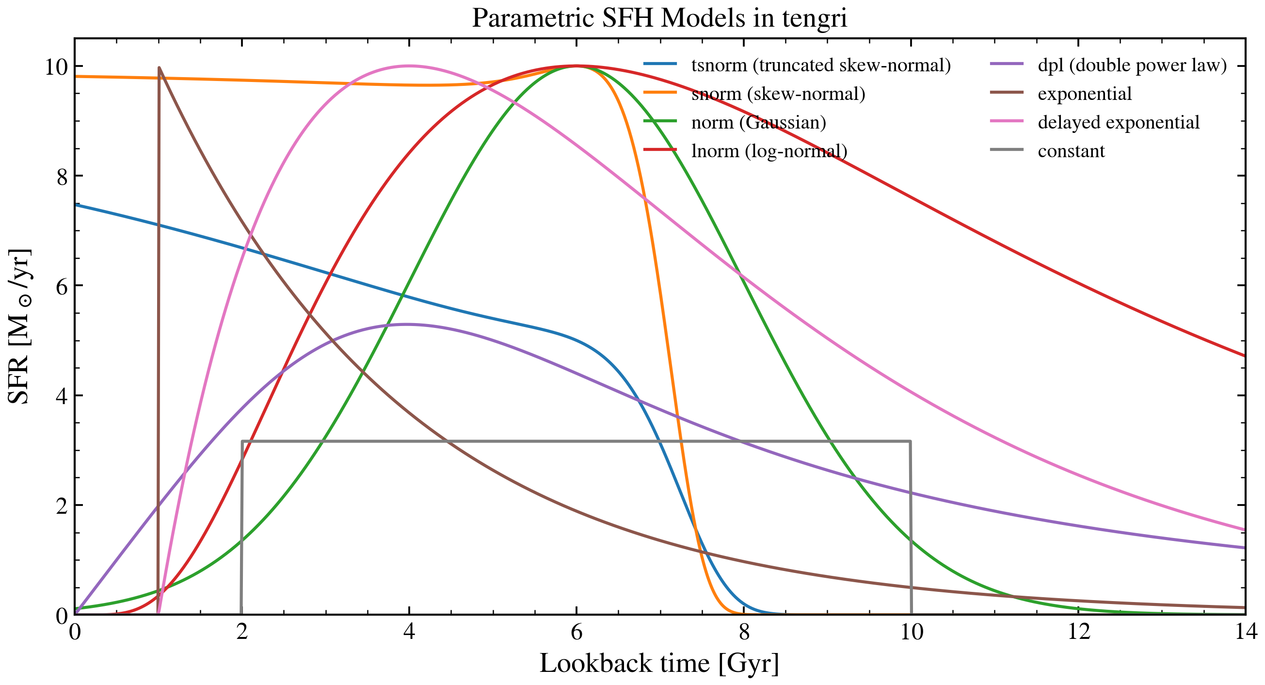
Parametric SFH Models

Compare all parametric star formation history models available in tengri. Each model is evaluated on a lookback-time grid and plotted with representative parameters. No SSP data required.

import jax.numpy as jnp
import matplotlib.pyplot as plt
import numpy as np

from tengri import (
    constant_sfh,
    delayed_exponential_sfh,
    dpl,
    exponential_sfh,
    lnorm,
    norm,
    snorm,
    tsnorm,
)
from tengri.analysis.plotting import setup_style

setup_style()


t_lookback = jnp.linspace(1e5, 14e9, 1000)
t_gyr = np.array(t_lookback) / 1e9

# --- Evaluate each SFH model with representative parameters ---
models = {
    "tsnorm (truncated skew-normal)": tsnorm(
        t_lookback, log_peak_sfr=1.0, peak_lbt=6e9, width=2e9, skew=1.0, trunc=3.0
    ),
    "snorm (skew-normal)": snorm(t_lookback, log_peak_sfr=1.0, peak_lbt=6e9, width=2e9, skew=1.5),
    "norm (Gaussian)": norm(t_lookback, log_peak_sfr=1.0, peak_lbt=6e9, width=2e9),
    "lnorm (log-normal)": lnorm(t_lookback, log_peak_sfr=1.0, peak_lbt=6e9, width=0.3),
    "dpl (double power law)": dpl(t_lookback, alpha=2.0, beta=1.0, tau=5e9, log_peak_sfr=1.0),
    "exponential": exponential_sfh(t_lookback, log_peak_sfr=1.0, tau=3e9, start=1e9),
    "delayed exponential": delayed_exponential_sfh(
        t_lookback, log_peak_sfr=1.0, tau=3e9, start=1e9
    ),
    "constant": constant_sfh(t_lookback, log_sfr=0.5, start=2e9, end=10e9),
}

colors = ["#1f77b4", "#ff7f0e", "#2ca02c", "#d62728", "#9467bd", "#8c564b", "#e377c2", "#7f7f7f"]

# --- Plot ---
fig, ax = plt.subplots(figsize=(9, 5))
for (name, sfr), color in zip(models.items(), colors):
    ax.plot(t_gyr, np.array(sfr), label=name, color=color, lw=1.5)

ax.set_xlabel("Lookback time [Gyr]")
ax.set_ylabel("SFR [M$_\\odot$/yr]")
ax.set_title("Parametric SFH Models in tengri")
ax.set_xlim(0, 14)
ax.set_ylim(0, None)
ax.legend(fontsize=10, frameon=False, ncol=2, loc="upper right")
fig.tight_layout()
plt.savefig("plot_parametric_sfh.png", dpi=150, bbox_inches="tight")
plt.show()