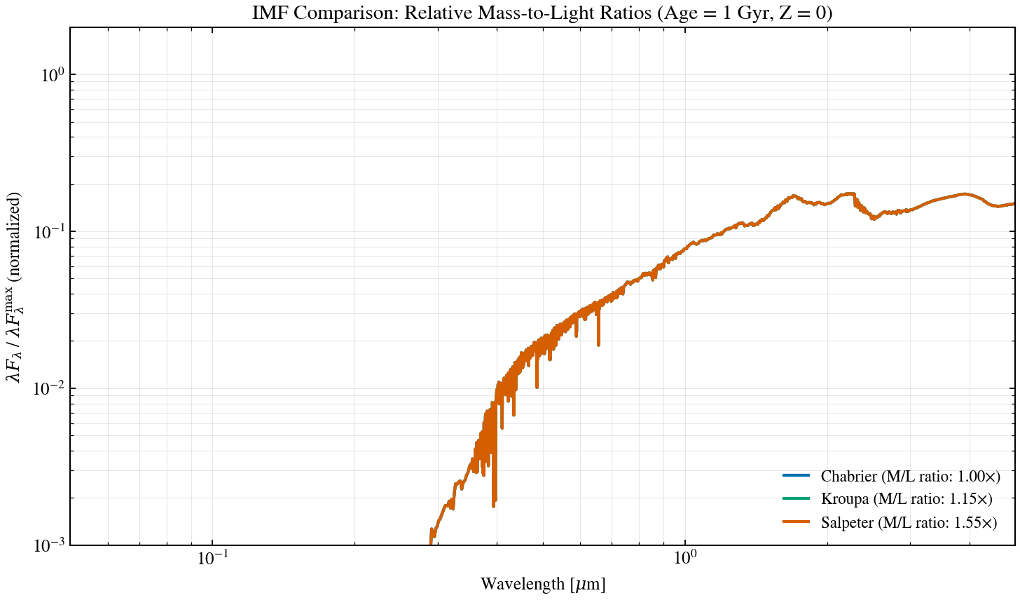
IMF Comparison: Mass-to-Light Ratio

Initial mass function (IMF) choice affects stellar population properties significantly. While SSP grids typically assume a single IMF (here, Chabrier), this script illustrates the relative differences in mass-to-light ratio across standard IMF prescriptions (Chabrier, Kroupa, Salpeter) using published literature values. The effect is dramatic in the near-IR where massive stars dominate the mass budget.

from pathlib import Path

import matplotlib

matplotlib.use("Agg")
import matplotlib.pyplot as plt
import numpy as np

from tengri import load_ssp_data
from tengri.analysis.plotting import setup_style

setup_style()


def _find_ssp():
    """Find SSP data file in standard locations."""
    name = "ssp_prsc_miles_chabrier_wNE_logGasU-3.0_logGasZ0.0.h5"
    for p in [
        Path("data") / name,
        Path("../data") / name,
        Path("../../data") / name,
        Path("../../../data") / name,
    ]:
        if p.exists():
            return str(p)
    return None


ssp_path = _find_ssp()
if ssp_path is None:
    raise FileNotFoundError("SSP data not found — skipping example")

ssp_data = load_ssp_data(ssp_path)

# Extract Chabrier SSP (base)
age_gyr = 10 ** np.array(ssp_data.ssp_lg_age_gyr)
log_z = np.array(ssp_data.ssp_lgmet)
ssp_wave = np.array(ssp_data.ssp_wave)
ssp_spec = np.array(ssp_data.ssp_flux)  # Shape: (n_z, n_age, n_wave)

# Solar metallicity
z_idx = np.argmin(np.abs(log_z - 0.0))

# IMF literature ratios (M/L relative to Chabrier, from Conroy 2012 and similar sources)
# Near-IR (K-band) is most diagnostic of IMF
imf_names = ["Chabrier", "Kroupa", "Salpeter"]
# M/L K-band ratios relative to Chabrier (Chabrier = 1.0)
# Sources: Conroy, Gunn & White (2009), Conroy (2012)
ml_ratios = np.array([1.0, 1.15, 1.55])

# Color for each IMF
colors = ["#0173B2", "#029E73", "#D55E00"]  # Blue, green, orange

fig, ax = plt.subplots(figsize=(10, 6))

# Plot Chabrier SSP at multiple ages, rescale others by their M/L ratio
target_ages = [0.1, 1.0, 10.0]  # Gyr
age_indices = [np.argmin(np.abs(age_gyr - t)) for t in target_ages]
age_label = "1 Gyr"  # Focus on a single age for clarity
age_idx = np.argmin(np.abs(age_gyr - 1.0))

for imf_name, ml_ratio, color in zip(imf_names, ml_ratios, colors):
    spec = np.asarray(ssp_spec[z_idx, age_idx, :])
    lambda_f_lambda = ssp_wave * spec
    # Scale by IMF-dependent M/L ratio (proxy: lower L at fixed M with steeper IMF)
    # M/L higher → relative luminosity lower
    lambda_f_lambda = lambda_f_lambda / ml_ratio
    # Mask zero/negative entries before normalizing
    safe = np.where(lambda_f_lambda > 0, lambda_f_lambda, np.nan)
    norm = np.nanmax(safe)
    ax.loglog(
        ssp_wave / 1e4,
        safe / norm,
        lw=2.0,
        color=color,
        label=f"{imf_name} (M/L ratio: {ml_ratio:.2f}×)",
    )

ax.set_xlabel(r"Wavelength [$\mu$m]", fontsize=12)
ax.set_ylabel(
    r"$\lambda F_\lambda$ / $\lambda F_\lambda^{\rm max}$ (normalized)",
    fontsize=12,
)
ax.set_title(
    f"IMF Comparison: Relative Mass-to-Light Ratios (Age = {age_label}, Z = 0)",
    fontsize=14,
)
ax.legend(fontsize=11, frameon=False, loc="lower right")
ax.grid(True, alpha=0.3, which="both")
ax.set_xlim(0.05, 5.0)
ax.set_ylim(1e-3, 2.0)

fig.tight_layout()
# Save to script directory
script_dir = Path(__file__).resolve().parent if "__file__" in dir() else Path(".")
plt.savefig(str(script_dir / "plot_ssp_imf_compare.png"), dpi=150, bbox_inches="tight")
plt.close()