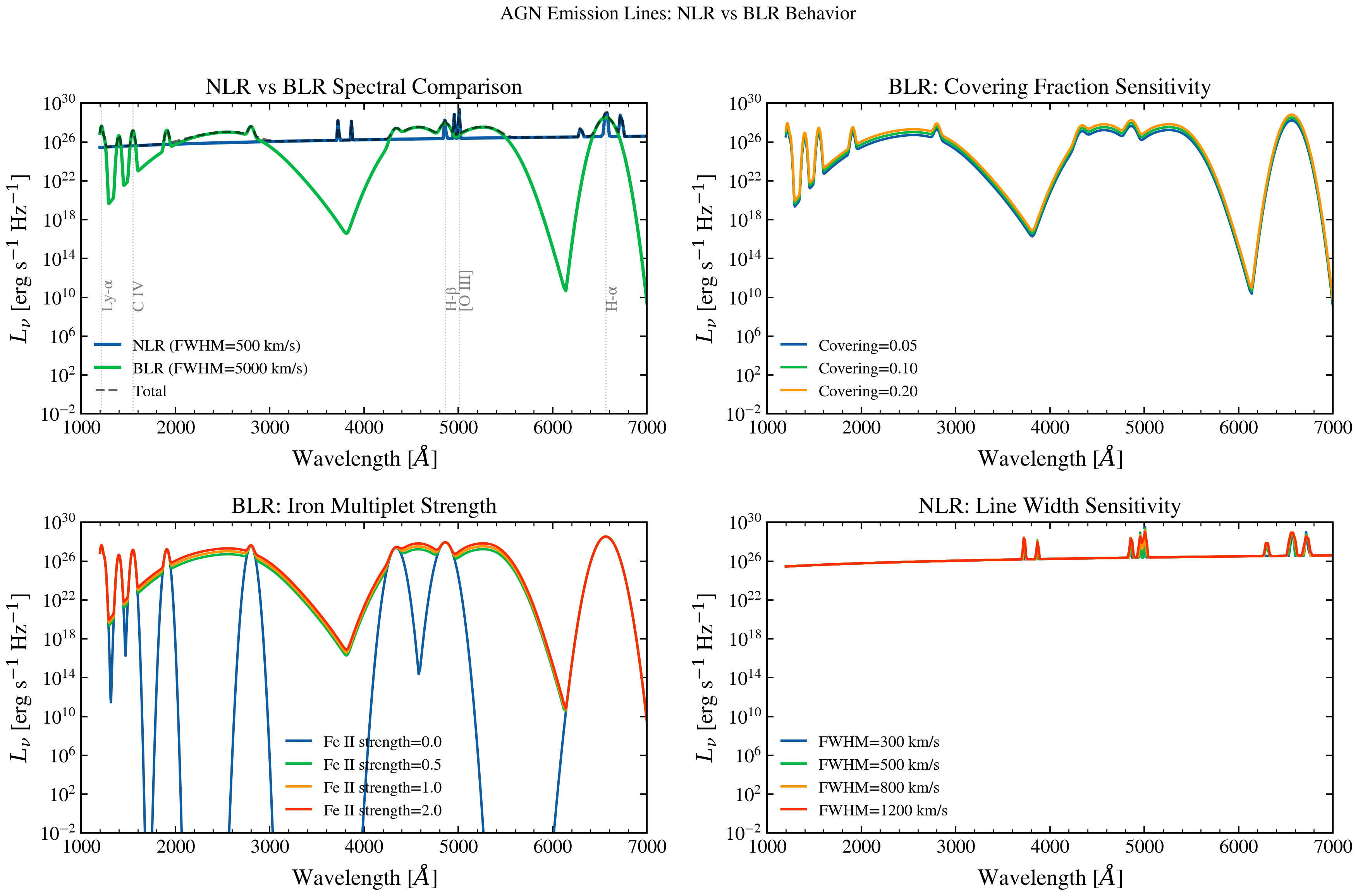
Narrow and Broad Line Region Emission

Plot narrow-line (NLR, FWHM ~500 km/s) and broad-line region (BLR, FWHM ~5000 km/s) emission spectra. Shows how BLR vanishes at high inclination angles (Type 2 AGN) while NLR remains visible.

import jax.numpy as jnp
import matplotlib.pyplot as plt
import numpy as np

from tengri.analysis.plotting import setup_style
from tengri.components.agn import compute_blr_sed, compute_nlr_sed

setup_style()

# Solar luminosity in cgs
LSUN_ERG = 3.828e33

# Wavelength grid: optical/UV
wavelength = jnp.logspace(np.log10(1200), np.log10(7000), 512)
wave_angstrom = np.array(wavelength)
wave_um = wave_angstrom / 1e4

fig, axes = plt.subplots(2, 2, figsize=(12, 8))

# Disc bolometric luminosity
L_disc_bol_erg = 10.0**44 * LSUN_ERG  # 10^44 L_sun

# --- Panel 1: NLR vs BLR at fixed covering fraction ---
ax = axes[0, 0]

covering_frac = 0.1
fwhm_nlr = 500.0
fwhm_blr = 5000.0

l_nlr = compute_nlr_sed(
    wavelength, l_disc_bol_erg=L_disc_bol_erg, covering_fraction=covering_frac, fwhm_kms=fwhm_nlr
)
l_blr = compute_blr_sed(
    wavelength,
    l_disc_bol_erg=L_disc_bol_erg,
    covering_fraction=covering_frac,
    fwhm_kms=fwhm_blr,
    agn_fe2_strength=1.0,
)

ax.semilogy(wave_angstrom, np.array(l_nlr) / LSUN_ERG, lw=2.0, label="NLR (FWHM=500 km/s)")
ax.semilogy(wave_angstrom, np.array(l_blr) / LSUN_ERG, lw=2.0, label="BLR (FWHM=5000 km/s)")
ax.semilogy(
    wave_angstrom,
    (np.array(l_nlr) + np.array(l_blr)) / LSUN_ERG,
    "k--",
    lw=1.5,
    alpha=0.6,
    label="Total",
)

# Mark key emission lines
lines = {"Ly-α": 1216, "C IV": 1549, "H-β": 4861, "[O III]": 5007, "H-α": 6563}
for lbl, wl in lines.items():
    ax.axvline(wl, color="gray", ls=":", alpha=0.5, lw=0.7)
    ax.text(wl, ax.get_ylim()[0] * 1.5, lbl, fontsize=10, rotation=90, color="gray", va="bottom")

ax.set_xlabel(r"Wavelength [$\AA$]")
ax.set_ylabel(r"$L_\nu$ [erg s$^{-1}$ Hz$^{-1}$]")
ax.set_title("NLR vs BLR Spectral Comparison")
ax.legend(fontsize=10, frameon=False)
ax.set_xlim(1000, 7000)
ax.set_ylim(1e-2, 1e30)

# --- Panel 2: BLR strength sweep ---
ax = axes[0, 1]

for covering_frac in [0.05, 0.10, 0.20]:
    l_blr = compute_blr_sed(
        wavelength,
        l_disc_bol_erg=L_disc_bol_erg,
        covering_fraction=covering_frac,
        fwhm_kms=5000.0,
        agn_fe2_strength=1.0,
    )
    label_txt = f"Covering={covering_frac:.2f}"
    ax.semilogy(wave_angstrom, np.array(l_blr) / LSUN_ERG, lw=1.5, label=label_txt)

ax.set_xlabel(r"Wavelength [$\AA$]")
ax.set_ylabel(r"$L_\nu$ [erg s$^{-1}$ Hz$^{-1}$]")
ax.set_title("BLR: Covering Fraction Sensitivity")
ax.legend(fontsize=10, frameon=False)
ax.set_xlim(1000, 7000)
ax.set_ylim(1e-2, 1e30)

# --- Panel 3: Fe II strength in BLR ---
ax = axes[1, 0]

covering_frac = 0.1
for fe2_strength in [0.0, 0.5, 1.0, 2.0]:
    l_blr = compute_blr_sed(
        wavelength,
        l_disc_bol_erg=L_disc_bol_erg,
        covering_fraction=covering_frac,
        fwhm_kms=5000.0,
        agn_fe2_strength=fe2_strength,
    )
    label_fe2 = f"Fe II strength={fe2_strength:.1f}"
    ax.semilogy(wave_angstrom, np.array(l_blr) / LSUN_ERG, lw=1.5, label=label_fe2)

ax.set_xlabel(r"Wavelength [$\AA$]")
ax.set_ylabel(r"$L_\nu$ [erg s$^{-1}$ Hz$^{-1}$]")
ax.set_title("BLR: Iron Multiplet Strength")
ax.legend(fontsize=10, frameon=False)
ax.set_xlim(1000, 7000)
ax.set_ylim(1e-2, 1e30)

# --- Panel 4: NLR FWHM variations ---
ax = axes[1, 1]

for fwhm in [300.0, 500.0, 800.0, 1200.0]:
    l_nlr = compute_nlr_sed(
        wavelength, l_disc_bol_erg=L_disc_bol_erg, covering_fraction=0.1, fwhm_kms=fwhm
    )
    ax.semilogy(wave_angstrom, np.array(l_nlr) / LSUN_ERG, lw=1.5, label=f"FWHM={fwhm:.0f} km/s")

ax.set_xlabel(r"Wavelength [$\AA$]")
ax.set_ylabel(r"$L_\nu$ [erg s$^{-1}$ Hz$^{-1}$]")
ax.set_title("NLR: Line Width Sensitivity")
ax.legend(fontsize=10, frameon=False)
ax.set_xlim(1000, 7000)
ax.set_ylim(1e-2, 1e30)

fig.suptitle("AGN Emission Lines: NLR vs BLR Behavior", fontsize=12)
fig.tight_layout(rect=[0, 0, 1, 0.97])
plt.savefig("plot_nlr_blr_lines.png", dpi=100, bbox_inches="tight")
plt.show()