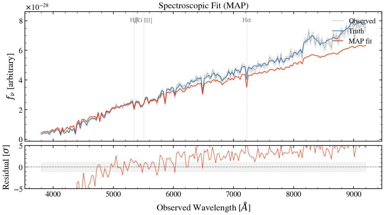
Spectroscopic SED Fit

Generate a mock galaxy spectrum and fit it with tengri’s MAP optimizer. Shows the observed and model spectra with a residual panel below.

from pathlib import Path

import jax
import jax.numpy as jnp
import matplotlib.pyplot as plt
import numpy as np

from tengri import (
    Fitter,
    Fixed,
    Observation,
    Parameters,
    SEDModel,
    Spectroscopy,
    Uniform,
    load_ssp_data,
)
from tengri.analysis.plotting import setup_style

setup_style()


# --- Check for SSP data ---
def _find_ssp():
    """Locate SSP data from project root or docs/ (sphinx-gallery) cwd."""
    name = "ssp_prsc_miles_chabrier_wNE_logGasU-3.0_logGasZ0.0.h5"
    for p in [
        Path("data") / name,
        Path("../data") / name,
        Path("../../data") / name,
        Path("../../../data") / name,
    ]:
        if p.exists():
            return str(p)
    return None


SSP_PATH = _find_ssp()
if SSP_PATH is None:
    raise FileNotFoundError("SSP data not found — skipping example")

# --- Setup ---
REDSHIFT = 0.1
WAVE_OBS = jnp.linspace(3800.0, 9200.0, 200)

ssp_data = load_ssp_data(SSP_PATH)
obs = Observation(
    spectroscopy=Spectroscopy(wave_obs=WAVE_OBS),
)

spec = Parameters(
    sfh_tsnorm_log_peak_sfr=Uniform(-1.0, 2.5),
    sfh_tsnorm_peak_lbt_gyr=Uniform(0.5, 12.0),
    sfh_tsnorm_width_gyr=Uniform(0.3, 5.0),
    sfh_tsnorm_skew=Uniform(-3.0, 3.0),
    sfh_tsnorm_trunc=Uniform(1.0, 10.0),
    met_logzsol=Uniform(-2.0, 0.2),
    dust_tau_bc=Fixed(0.3),
    dust_tau_diff=Fixed(0.2),
    dust_slope=Fixed(-0.7),
    redshift=Fixed(REDSHIFT),
)
model = SEDModel(spec, ssp_data, observation=obs)

# --- Generate mock spectrum ---
true_params = spec.sample(jax.random.PRNGKey(42))
mock = model.mock_spectrum(true_params, WAVE_OBS, snr=30.0, key=jax.random.PRNGKey(1))

# --- Fit with MAP ---
fitter = Fitter(model, mock.flux_obs, mock.noise, data_type="spectroscopy")
posterior = fitter.run("map", optimizer="adam", n_steps=500, verbose=False)
best_spec = model.predict_spectrum(posterior.params, WAVE_OBS)

# --- Plot ---
wave = np.array(WAVE_OBS)
fig, (ax, ax_res) = plt.subplots(
    2, 1, figsize=(10, 5), height_ratios=[3, 1], sharex=True, gridspec_kw={"hspace": 0.05}
)

ax.plot(wave, np.array(mock.flux_obs), color="0.6", lw=0.5, label="Observed")
ax.fill_between(
    wave,
    np.array(mock.flux_obs - mock.noise),
    np.array(mock.flux_obs + mock.noise),
    color="0.85",
    alpha=0.6,
)
ax.plot(wave, np.array(mock.flux_true), "C0-", lw=1.2, label="Truth", alpha=0.7)
ax.plot(wave, np.array(best_spec), "C3-", lw=1.0, label="MAP fit")
ax.set_ylabel(r"$f_\nu$ [arbitrary]")
ax.legend(frameon=False, loc="upper right")
ax.set_title("Spectroscopic Fit (MAP)")

# Spectral feature labels
features = {"H$\\beta$": 4861, "[O III]": 5007, "H$\\alpha$": 6563}
for name, lam_rest in features.items():
    lam_obs = lam_rest * (1 + REDSHIFT)
    if wave[0] < lam_obs < wave[-1]:
        ax.axvline(lam_obs, ls=":", color="grey", lw=0.6, alpha=0.5)
        ax.text(lam_obs, ax.get_ylim()[1] * 0.92, name, fontsize=10, ha="center", color="grey")

residuals = (np.array(mock.flux_obs) - np.array(best_spec)) / np.array(mock.noise)
ax_res.axhline(0, color="0.5", ls="--", lw=0.8)
ax_res.plot(wave, residuals, "C3-", lw=0.6)
ax_res.fill_between(wave, -1, 1, color="0.9", alpha=0.5)
ax_res.set_xlabel(r"Observed Wavelength [$\AA$]")
ax_res.set_ylabel(r"Residual [$\sigma$]")
ax_res.set_ylim(-5, 5)

fig.tight_layout()
plt.savefig("plot_spectrum_fit.png", dpi=150, bbox_inches="tight")
plt.show()