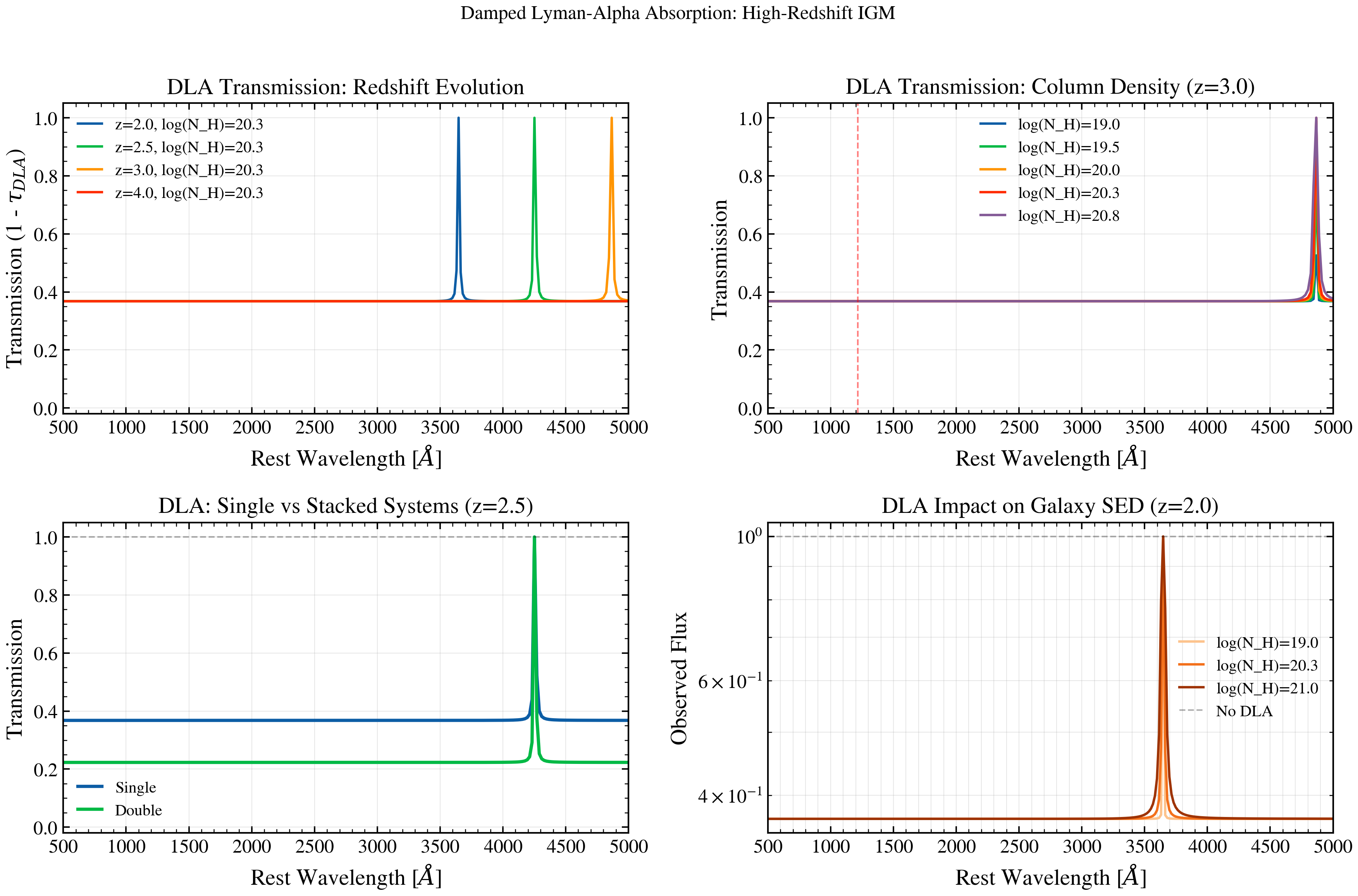
Damped Lyman-Alpha (DLA) Absorption

Plot DLA transmission curves at high redshift (z > 2), showing Lyman-alpha forest absorption and strong DLA features that sculpt the UV-to-optical SED. Demonstrates wavelength-dependent attenuation.

import jax.numpy as jnp
import matplotlib.pyplot as plt
import numpy as np

from tengri import dla_transmission_obs
from tengri.analysis.plotting import setup_style

setup_style()

# Wavelength grid: UV to optical
wavelength_rest = jnp.logspace(np.log10(500), np.log10(5000), 512)  # Angstrom

fig, axes = plt.subplots(2, 2, figsize=(12, 8))

# --- Panel 1: DLA transmission at different redshifts ---
ax = axes[0, 0]

log_nh_col = 20.3  # DLA column density
for z in [2.0, 2.5, 3.0, 4.0]:
    # Transmission in observed frame
    tau_dla = dla_transmission_obs(wavelength_rest, z_dla=z, log_n_hi=log_nh_col)
    transmission = jnp.exp(-tau_dla)

    ax.plot(
        np.array(wavelength_rest),
        np.array(transmission),
        lw=1.5,
        label=f"z={z:.1f}, log(N_H)={log_nh_col:.1f}",
    )

ax.set_xlabel(r"Rest Wavelength [$\AA$]")
ax.set_ylabel(r"Transmission (1 - $\tau_{DLA}$)")
ax.set_title("DLA Transmission: Redshift Evolution")
ax.legend(fontsize=10, frameon=False)
ax.set_xlim(500, 5000)
ax.set_ylim(-0.02, 1.05)
ax.grid(True, alpha=0.3)

# --- Panel 2: Column density dependence (Lyman-alpha forest) ---
ax = axes[0, 1]

z = 3.0
for log_nh in [19.0, 19.5, 20.0, 20.3, 20.8]:
    tau_dla = dla_transmission_obs(wavelength_rest, z_dla=z, log_n_hi=log_nh)
    transmission = jnp.exp(-tau_dla)

    ax.plot(
        np.array(wavelength_rest),
        np.array(transmission),
        lw=1.5,
        label=f"log(N_H)={log_nh:.1f}",
    )

ax.set_xlabel(r"Rest Wavelength [$\AA$]")
ax.set_ylabel(r"Transmission")
ax.set_title(f"DLA Transmission: Column Density (z={z})")
ax.legend(fontsize=10, frameon=False)
ax.set_xlim(500, 5000)
ax.set_ylim(-0.02, 1.05)
ax.grid(True, alpha=0.3)

# Mark Lyman-alpha
ax.axvline(1216, color="red", ls="--", lw=1.0, alpha=0.5, label="Ly-α")

# --- Panel 3: Multiple DLAs (stacked systems) ---
ax = axes[1, 0]

z = 2.5
# Single DLA
tau_single = dla_transmission_obs(wavelength_rest, z_dla=z, log_n_hi=20.3)
transmission_single = jnp.exp(-tau_single)

# Approximate double DLA (stack two with slightly different optical depths)
tau_double = 1.5 * tau_single  # Rough stacking approximation
transmission_double = jnp.exp(-tau_double)

ax.plot(np.array(wavelength_rest), np.array(transmission_single), lw=2.0, label="Single")
ax.plot(np.array(wavelength_rest), np.array(transmission_double), lw=2.0, label="Double")
trans_none = np.ones_like(transmission_single)
ax.plot(np.array(wavelength_rest), trans_none, "k--", lw=1.0, alpha=0.3)

ax.set_xlabel(r"Rest Wavelength [$\AA$]")
ax.set_ylabel(r"Transmission")
ax.set_title(f"DLA: Single vs Stacked Systems (z={z})")
ax.legend(fontsize=10, frameon=False)
ax.set_xlim(500, 5000)
ax.set_ylim(-0.02, 1.05)
ax.grid(True, alpha=0.3)

# --- Panel 4: Attenuation impact on galaxy SED ---
ax = axes[1, 1]

z = 2.0
log_nh_values = [19.0, 20.3, 21.0]
colors = plt.cm.Oranges(np.linspace(0.3, 0.9, len(log_nh_values)))

# Mock galaxy SED (assume constant rest-frame SED)
galaxy_sed = np.ones_like(wavelength_rest)  # Flat SED in L_nu

for log_nh, color in zip(log_nh_values, colors):
    tau_dla = dla_transmission_obs(wavelength_rest, z_dla=z, log_n_hi=log_nh)
    transmission = jnp.exp(-tau_dla)
    attenuated_sed = galaxy_sed * np.array(transmission)

    ax.semilogy(
        np.array(wavelength_rest),
        attenuated_sed,
        lw=1.5,
        label=f"log(N_H)={log_nh:.1f}",
        color=color,
    )

ax.semilogy(np.array(wavelength_rest), galaxy_sed, "k--", lw=1.0, alpha=0.3, label="No DLA")
ax.set_xlabel(r"Rest Wavelength [$\AA$]")
ax.set_ylabel(r"Observed Flux")
ax.set_title(f"DLA Impact on Galaxy SED (z={z})")
ax.legend(fontsize=10, frameon=False)
ax.set_xlim(500, 5000)
ax.grid(True, alpha=0.3, which="both")

fig.suptitle("Damped Lyman-Alpha Absorption: High-Redshift IGM", fontsize=12)
fig.tight_layout(rect=[0, 0, 1, 0.97])
plt.savefig("plot_dla_absorption.png", dpi=100, bbox_inches="tight")
plt.show()