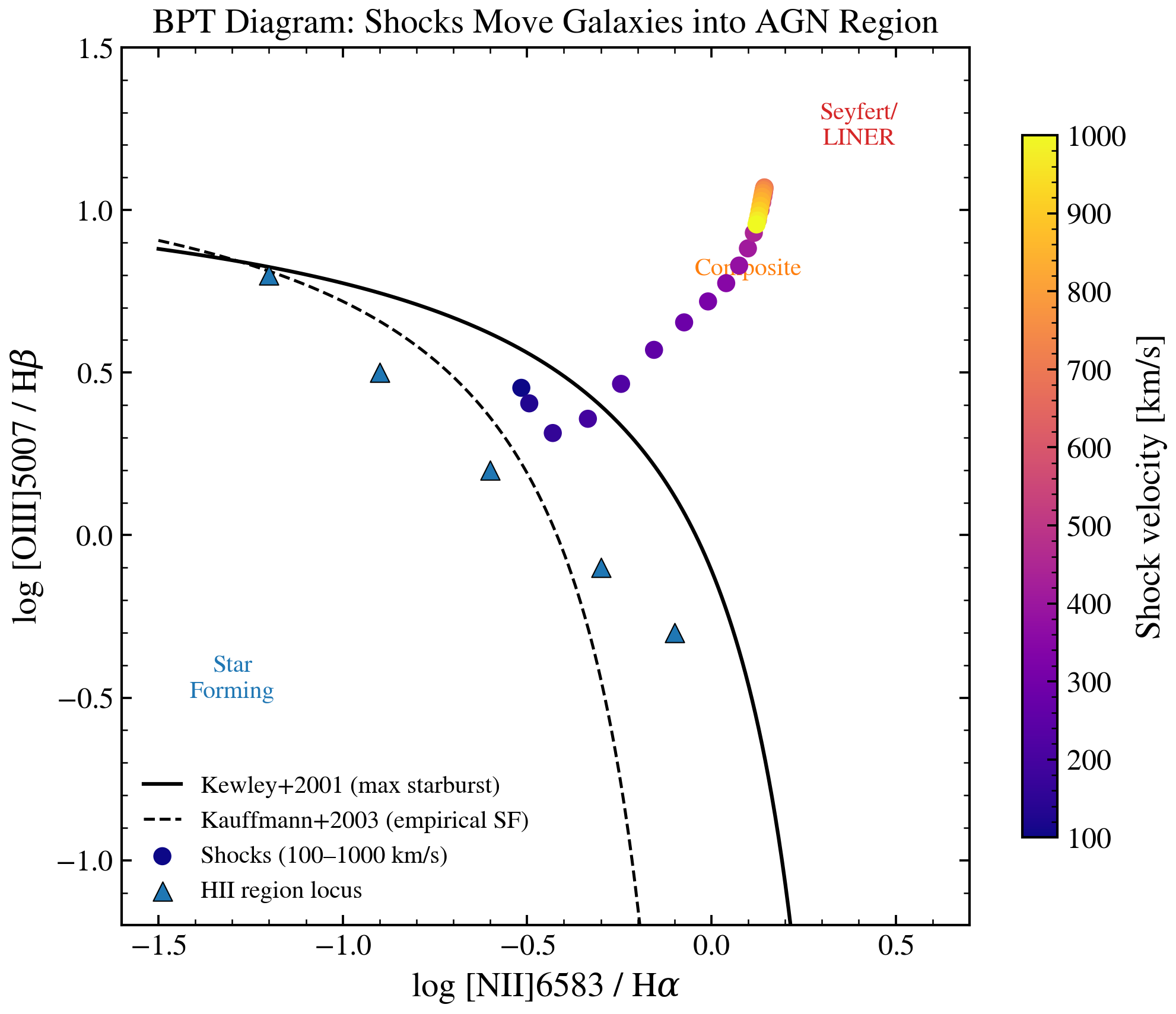
BPT Diagnostics: Star Formation, Shocks, and AGN

The BPT diagram ([OIII]/Hβ vs [NII]/Hα) separates three sources of ionizing photons. Shocks (MAPPINGS V, Allen+2008) move emission-line galaxies into the composite and Seyfert regions as shock velocity increases.

import matplotlib.pyplot as plt
import numpy as np

from tengri import setup_style
from tengri.nebular import shock_line_ratios

setup_style()

# --- Kewley+2001 maximum starburst line ---
log_nii_ha_grid = np.linspace(-1.5, 0.3, 200)
log_oiii_hb_kewley = 0.61 / (log_nii_ha_grid - 0.47) + 1.19

# --- Kauffmann+2003 empirical SF line ---
log_oiii_hb_kauff = 0.61 / (log_nii_ha_grid - 0.05) + 1.3

# --- Shock track: velocity 100 → 1000 km/s ---
velocities = np.linspace(100.0, 1000.0, 30)
shock_nii_ha = []
shock_oiii_hb = []
for v in velocities:
    r = shock_line_ratios(float(v))
    ha = float(r["HA_6563A"])
    hb = float(r.get("Hb_4861A", ha / 2.86))
    nii = float(r["NII_6583A"])
    oiii = float(r["O3_5007A"])
    if ha > 0 and hb > 0:
        shock_nii_ha.append(np.log10(nii / ha))
        shock_oiii_hb.append(np.log10(max(oiii / hb, 1e-10)))

# --- Typical HII region locus ---
hii_nii_ha = np.array([-1.2, -0.9, -0.6, -0.3, -0.1])
hii_oiii_hb = np.array([0.8, 0.5, 0.2, -0.1, -0.3])

fig, ax = plt.subplots(figsize=(7, 6))

# Demarcation lines
mask_k = log_nii_ha_grid < 0.47
ax.plot(
    log_nii_ha_grid[mask_k],
    log_oiii_hb_kewley[mask_k],
    "k-",
    lw=1.5,
    label="Kewley+2001 (max starburst)",
)
mask_kauff = log_nii_ha_grid < 0.05
ax.plot(
    log_nii_ha_grid[mask_kauff],
    log_oiii_hb_kauff[mask_kauff],
    "k--",
    lw=1.2,
    label="Kauffmann+2003 (empirical SF)",
)

# Region labels
ax.text(-1.3, -0.5, "Star\nForming", fontsize=10, color="#1f77b4", ha="center")
ax.text(0.1, 0.8, "Composite", fontsize=10, color="#ff7f0e", ha="center")
ax.text(0.4, 1.2, "Seyfert/\nLINER", fontsize=10, color="#d62728", ha="center")

# Shock track
if shock_nii_ha:
    sc = ax.scatter(
        shock_nii_ha,
        shock_oiii_hb,
        c=velocities[: len(shock_nii_ha)],
        cmap="plasma",
        s=40,
        zorder=5,
        label="Shocks (100–1000 km/s)",
    )
    plt.colorbar(sc, ax=ax, label="Shock velocity [km/s]", shrink=0.8)

# HII locus
ax.scatter(
    hii_nii_ha,
    hii_oiii_hb,
    color="#1f77b4",
    s=60,
    marker="^",
    label="HII region locus",
    zorder=6,
    edgecolors="k",
    lw=0.5,
)

ax.set_xlabel(r"log [NII]6583 / H$\alpha$")
ax.set_ylabel(r"log [OIII]5007 / H$\beta$")
ax.set_title("BPT Diagram: Shocks Move Galaxies into AGN Region")
ax.set_xlim(-1.6, 0.7)
ax.set_ylim(-1.2, 1.5)
ax.legend(fontsize=10, frameon=False, loc="lower left")
fig.tight_layout()
plt.savefig("plot_bpt_diagnostics.png", dpi=150, bbox_inches="tight")
plt.show()