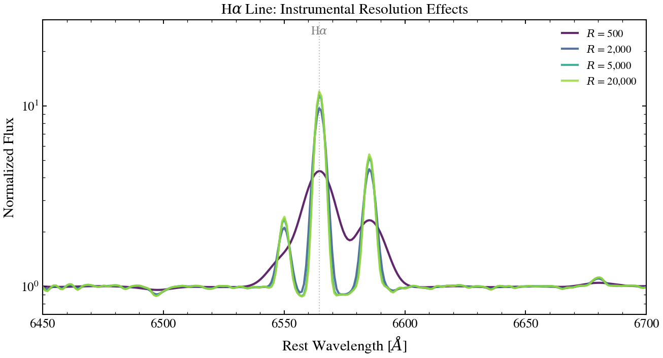
Instrumental Resolution Sweep

Sweep instrumental resolution R ∈ {500, 2000, 5000, 20000} to demonstrate how spectral resolution affects line profile visibility. The Hα line (~6564.6 Å vacuum) transforms from a single broad bump to a sharply resolved absorption feature as resolution increases. High-res spectroscopy reveals kinematics.

from pathlib import Path

import jax.numpy as jnp
import matplotlib.pyplot as plt
import numpy as np
from scipy.ndimage import gaussian_filter1d

from tengri import Fixed, Observation, Parameters, SEDModel, Spectroscopy, load_ssp_data
from tengri.analysis.plotting import setup_style

setup_style()


def _find_ssp():
    """Locate SSP data from project root or docs/ (sphinx-gallery) cwd."""
    name = "ssp_prsc_miles_chabrier_wNE_logGasU-3.0_logGasZ0.0.h5"
    for p in [
        Path("data") / name,
        Path("../data") / name,
        Path("../../data") / name,
        Path("../../../data") / name,
    ]:
        if p.exists():
            return str(p)
    return None


SSP_PATH = _find_ssp()
if SSP_PATH is None:
    raise FileNotFoundError("SSP data not found — skipping example")

# --- Setup ---
ssp_data = load_ssp_data(SSP_PATH)
WAVE_OBS = jnp.linspace(6000.0, 7100.0, 400)
REDSHIFT = 0.1

obs = Observation(
    spectroscopy=Spectroscopy(wave_obs=WAVE_OBS),
)

spec = Parameters(
    sfh_tsnorm_log_peak_sfr=Fixed(0.5),
    sfh_tsnorm_peak_lbt_gyr=Fixed(1.5),
    sfh_tsnorm_width_gyr=Fixed(1.2),
    sfh_tsnorm_skew=Fixed(-0.2),
    sfh_tsnorm_trunc=Fixed(2.0),
    met_logzsol=Fixed(0.1),
    dust_tau_bc=Fixed(0.2),
    dust_tau_diff=Fixed(0.1),
    dust_slope=Fixed(-0.7),
    redshift=Fixed(REDSHIFT),
)
model = SEDModel(spec, ssp_data, observation=obs)

# --- Predict rest-frame spectrum ---
pred = model.predict_rest_sed({})
wave_rest = np.asarray(pred.wavelength)
sed_rest = np.asarray(pred.sed)

# --- Zoom to Hα region in the rest frame ---
# wave_rest is already rest-frame Å from predict_rest_sed; no division by
# (1+z) needed (that would double-blueshift and offset Hα by ~80 Å).
zoom_mask = (wave_rest >= 6400) & (wave_rest <= 6750)
wave_zoom = wave_rest[zoom_mask]
sed_zoom = sed_rest[zoom_mask]

# Normalize to continuum level
sed_zoom = sed_zoom / np.median(sed_zoom)

# --- Resolution sweep (R = λ / Δλ) ---
resolution_vals = [500, 2000, 5000, 20000]
colors = plt.cm.viridis(np.linspace(0.0, 0.85, len(resolution_vals)))

# Wavelength pixel width
dlam_pix = np.mean(np.diff(wave_zoom))

fig, ax = plt.subplots(figsize=(9, 5))

for r, color in zip(resolution_vals, colors):
    # Wavelength resolution element from R
    dlam = np.mean(wave_zoom) / r
    sigma_pix = dlam / (2.355 * dlam_pix)  # FWHM → sigma

    # Apply Gaussian broadening
    sed_conv = gaussian_filter1d(sed_zoom, sigma=sigma_pix)

    ax.plot(
        wave_zoom,
        sed_conv,
        lw=2.0,
        color=color,
        label=f"$R$ = {r:,}",
        alpha=0.85,
    )

# Set limits FIRST so the H-alpha annotation places at the right y-coord.
ax.set_xlabel(r"Rest Wavelength [$\AA$]")
ax.set_ylabel("Normalized Flux")
ax.set_title(r"H$\alpha$ Line: Instrumental Resolution Effects")
# Zoom out enough to show the full Hα + [N II] λλ6549,6585 complex with
# continuum context either side. Log-y keeps the bright emission peaks on
# the same panel as the ~1% absorption-line wiggles in the continuum.
ax.set_xlim(6450, 6700)
ax.set_yscale("log")
ax.set_ylim(0.7, 30.0)

# Mark Hα center (vacuum) using axis-fraction transform so the text always
# anchors to the visible top of the panel regardless of data range.
ha_center = 6564.61
ax.axvline(ha_center, ls=":", lw=1.0, color="grey", alpha=0.5)
ax.text(
    ha_center,
    0.95,
    r"H$\alpha$",
    fontsize=11,
    ha="center",
    color="grey",
    transform=ax.get_xaxis_transform(),
)
ax.legend(frameon=False, loc="upper right", fontsize=10)
fig.tight_layout()
plt.savefig("plot_resolution_sweep.png", dpi=150, bbox_inches="tight")
plt.show()