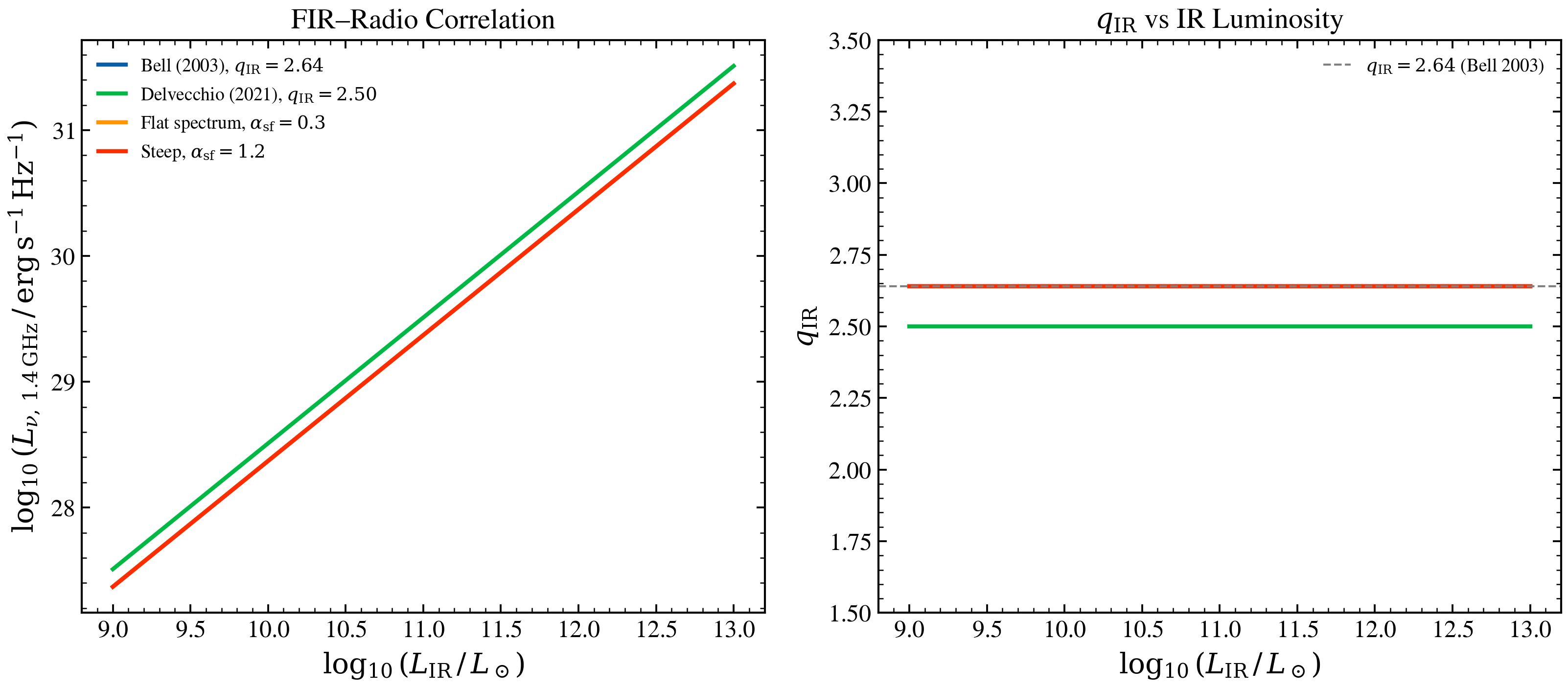
FIR–Radio Correlation

The FIR–radio correlation (van der Kruit 1971; Helou et al. 1985) is one of the tightest empirical relations in galaxy physics, holding over five decades in luminosity. Parameterized by \(q_{\rm IR}\):

\[q_{\rm IR} = \log_{10}\!\left(\frac{L_{\rm IR}}{3.75\times10^{12}\,{\rm Hz}}\right) - \log_{10}\!\left(L_{\nu,\,1.4\,{\rm GHz}}\right)\]

This example sweeps \(L_{\rm IR}\) from \(10^{9}\) to \(10^{13}\,L_{\odot}\) for four radio calibrations, recovering the expected tight linear correlation and showing how the \(q_{\rm IR}\) parameter shifts the normalization.

import jax
import jax.numpy as jnp
import matplotlib.pyplot as plt
import numpy as np

jax.config.update("jax_enable_x64", True)

from tengri.analysis.plotting import setup_style
from tengri.radio import radio_star_forming

setup_style()

# 1.4 GHz reference wavelength in Angstrom
_C_LIGHT = 2.99792458e18  # Å/s
NU_1P4GHZ = 1.4e9  # Hz
WAVE_1P4GHZ = _C_LIGHT / NU_1P4GHZ  # Å

# Sweep IR luminosity
log_lir_lsun = np.linspace(9, 13, 60)
_L_SUN_ERG = 3.839e33
L_ir_erg = 10**log_lir_lsun * _L_SUN_ERG

# Radio calibrations to compare
calibrations = [
    {"label": r"Bell (2003), $q_{\rm IR}=2.64$", "q_ir": 2.64, "alpha": 0.8, "color": "C0"},
    {"label": r"Delvecchio (2021), $q_{\rm IR}=2.50$", "q_ir": 2.50, "alpha": 0.8, "color": "C1"},
    {"label": r"Flat spectrum, $\alpha_{\rm sf}=0.3$", "q_ir": 2.64, "alpha": 0.3, "color": "C2"},
    {"label": r"Steep, $\alpha_{\rm sf}=1.2$", "q_ir": 2.64, "alpha": 1.2, "color": "C3"},
]

fig, axes = plt.subplots(1, 2, figsize=(11, 5))
ax_corr, ax_qir = axes

wave_ref = jnp.array([WAVE_1P4GHZ])

for cal in calibrations:
    l_radio_arr = []
    for lir in L_ir_erg:
        l_nu_arr = radio_star_forming(
            wave_ref, L_ir=float(lir), q_ir=cal["q_ir"], alpha_sf=cal["alpha"]
        )
        l_radio_arr.append(float(np.asarray(l_nu_arr).ravel()[0]))
    l_radio = np.array(l_radio_arr)

    # FIR–radio correlation
    log_l_radio = np.log10(np.maximum(l_radio, 1e10))
    ax_corr.plot(log_lir_lsun, log_l_radio, color=cal["color"], lw=2.0, label=cal["label"])

    # q_IR = log10(L_IR / 3.75e12 Hz) - log10(L_nu,1.4GHz)   [Helou+ 1985]
    log_l_ir_erg = np.log10(L_ir_erg)
    q_ir_vals = log_l_ir_erg - np.log10(3.75e12) - log_l_radio
    ax_qir.plot(log_lir_lsun, q_ir_vals, color=cal["color"], lw=2.0)

ax_corr.set_xlabel(r"$\log_{10}(L_{\rm IR}\,/\,L_\odot)$")
ax_corr.set_ylabel(r"$\log_{10}(L_{\nu,\,1.4\,{\rm GHz}}\,/\,{\rm erg\,s^{-1}\,Hz^{-1}})$")
ax_corr.set_title("FIR–Radio Correlation")
ax_corr.legend(frameon=False, fontsize=9)

ax_qir.axhline(2.64, color="0.5", ls="--", lw=1.0, label=r"$q_{\rm IR}=2.64$ (Bell 2003)")
ax_qir.set_xlabel(r"$\log_{10}(L_{\rm IR}\,/\,L_\odot)$")
ax_qir.set_ylabel(r"$q_{\rm IR}$")
ax_qir.set_title(r"$q_{\rm IR}$ vs IR Luminosity")
ax_qir.legend(frameon=False, fontsize=9)
ax_qir.set_ylim(1.5, 3.5)

fig.tight_layout()
plt.savefig("plot_fir_radio_correlation.png", dpi=150, bbox_inches="tight")
plt.show()