Note
Go to the end to download the full example code.
MAPPINGS V shocks: velocity, density, and magnetic field effects
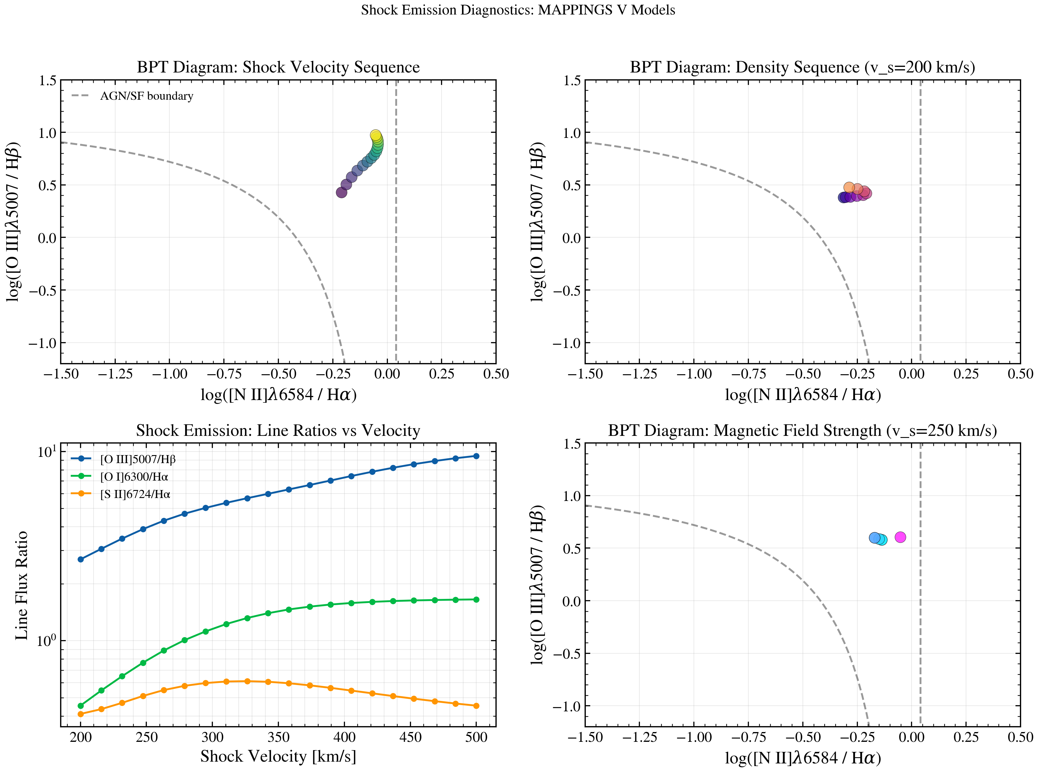
Shock emission (MAPPINGS V models) can mimic AGN on the BPT diagram. We show how shock velocity, gas density, and magnetic field strength affect line ratios and diagnostic positions. Four-panel layout shows velocity and density sequences on BPT, line ratios vs velocity, and magnetic field strength.
import os

os.environ["TF_CPP_MIN_LOG_LEVEL"] = "2"  # suppress XLA/PjRt C++ INFO+WARNING logs

import warnings

import matplotlib.pyplot as plt
import numpy as np

from tengri.nebular import shock_line_ratios
from tengri.plot import setup_style

setup_style()
warnings.filterwarnings("ignore", message=".*deprecated.*")

fig, axes = plt.subplots(2, 2, figsize=(11, 9))

# A single (v, n, B) corner falling outside the MAPPINGS V grid raises, and
# skipping it is correct. Every point of a sweep failing is not: each BPT panel
# below also draws a reference boundary curve *outside* its try block, so the
# axes still holds 100 points and no figure-level "is this blank?" check can
# tell an empty sweep from a full one. Only the loop knows. Each panel counts
# what it drew and calls _guard.
_failures: list[Exception] = []


def _guard(n_drawn: int, n_tried: int, panel: str) -> None:
    """Fail loudly when a panel's entire sweep was swallowed."""
    if n_drawn:
        return
    first = _failures[0] if _failures else None
    raise RuntimeError(
        f"{panel}: all {n_tried} shock models failed, so this panel shows only "
        f"its reference curve. First failure: {type(first).__name__}: {first}"
    ) from first


ax = axes[0, 0]
v_shock_range = np.linspace(200, 500, 15)
colors = plt.cm.viridis(np.linspace(0, 1, len(v_shock_range)))

drawn = 0
for v_shock, color in zip(v_shock_range, colors):
    try:
        line_ratios = shock_line_ratios(
            shock_velocity=float(v_shock),
            shock_log_density=2.0,
            shock_b_over_sqrt_n=1.0,
        )
        log_oiii_hb = np.log10(line_ratios["O3_5007A"] / line_ratios["Hb_4861A"])
        log_nii_ha = np.log10(line_ratios["NII_6583A"] / line_ratios["HA_6563A"])
        ax.scatter(log_nii_ha, log_oiii_hb, color=color, s=80, alpha=0.7, edgecolors="k", lw=0.3)
        drawn += 1
    except Exception as e:
        _failures.append(e)

_guard(drawn, len(v_shock_range), "BPT velocity sweep")

x_bpt = np.linspace(-1.5, 0.5, 100)
y_bpt_agn = 0.61 / (x_bpt - 0.05) + 1.3
ax.plot(x_bpt, y_bpt_agn, "k--", lw=1.5, alpha=0.4, label="AGN/SF boundary")
ax.set_xlabel(r"$\log$ [NII] / H$\alpha$")
ax.set_ylabel(r"$\log$ [OIII] / H$\beta$")
ax.set_title("BPT: Shock Velocity (200–500 km/s)")
ax.grid(True, alpha=0.3)
ax.legend(fontsize=10, frameon=False)
ax.set_xlim(-1.5, 0.5)
ax.set_ylim(-1.2, 1.5)

ax = axes[0, 1]
density_range = np.logspace(0, 4, 12)
colors = plt.cm.plasma(np.linspace(0, 1, len(density_range)))

drawn = 0
for dens, color in zip(density_range, colors):
    try:
        line_ratios = shock_line_ratios(
            shock_velocity=200.0,
            shock_log_density=float(np.log10(dens)),
            shock_b_over_sqrt_n=1.0,
        )
        log_oiii_hb = np.log10(line_ratios["O3_5007A"] / line_ratios["Hb_4861A"])
        log_nii_ha = np.log10(line_ratios["NII_6583A"] / line_ratios["HA_6563A"])
        ax.scatter(log_nii_ha, log_oiii_hb, color=color, s=80, alpha=0.7, edgecolors="k", lw=0.3)
        drawn += 1
    except Exception as e:
        _failures.append(e)

_guard(drawn, len(density_range), "BPT density sweep")

ax.plot(x_bpt, y_bpt_agn, "k--", lw=1.5, alpha=0.4)
ax.set_xlabel(r"$\log$ [NII] / H$\alpha$")
ax.set_ylabel(r"$\log$ [OIII] / H$\beta$")
ax.set_title("BPT: Density (200 km/s)")
ax.grid(True, alpha=0.3)
ax.set_xlim(-1.5, 0.5)
ax.set_ylim(-1.2, 1.5)

ax = axes[1, 0]
v_shock_dense = np.linspace(200, 500, 20)
line_flux_dict = {
    "[OIII]/Hβ": [],
    "[OI]/Hα": [],
    "[SII]/Hα": [],
}

for v_shock in v_shock_dense:
    try:
        line_ratios = shock_line_ratios(
            shock_velocity=float(v_shock),
            shock_log_density=2.0,
            shock_b_over_sqrt_n=1.0,
        )
        line_flux_dict["[OIII]/Hβ"].append(line_ratios["O3_5007A"] / line_ratios["Hb_4861A"])
        line_flux_dict["[OI]/Hα"].append(line_ratios["OI_6300A"] / line_ratios["HA_6563A"])
        line_flux_dict["[SII]/Hα"].append(
            (line_ratios["SII_6716A"] + line_ratios["SII_6731A"]) / line_ratios["HA_6563A"]
        )
    except Exception as e:
        _failures.append(e)

# This panel plots nothing at all when the sweep is empty (the `if ratios:`
# below is False for every series), so it fails silent rather than blank.
_guard(len(line_flux_dict["[OIII]/Hβ"]), len(v_shock_dense), "line-ratio vs velocity")

for label, ratios in line_flux_dict.items():
    if ratios:
        ax.semilogy(v_shock_dense[: len(ratios)], ratios, "o-", lw=1.5, label=label, markersize=4)

ax.set_xlabel("Shock Velocity [km/s]")
ax.set_ylabel("Line Flux Ratio")
ax.legend(fontsize=10, frameon=False)
ax.grid(True, alpha=0.3, which="both")

ax = axes[1, 1]
b_param_range = np.logspace(-3, 1, 12)
colors = plt.cm.cool(np.linspace(0, 1, len(b_param_range)))

drawn = 0
for b_param, color in zip(b_param_range, colors):
    try:
        line_ratios = shock_line_ratios(
            shock_velocity=250.0,
            shock_log_density=2.0,
            shock_b_over_sqrt_n=float(max(b_param, 1e-4)),
        )
        log_oiii_hb = np.log10(line_ratios["O3_5007A"] / line_ratios["Hb_4861A"])
        log_nii_ha = np.log10(line_ratios["NII_6583A"] / line_ratios["HA_6563A"])
        ax.scatter(log_nii_ha, log_oiii_hb, color=color, s=80, alpha=0.7, edgecolors="k", lw=0.3)
        drawn += 1
    except Exception as e:
        _failures.append(e)

_guard(drawn, len(b_param_range), "BPT magnetic-field sweep")

ax.plot(x_bpt, y_bpt_agn, "k--", lw=1.5, alpha=0.4)
ax.set_xlabel(r"$\log$ [NII] / H$\alpha$")
ax.set_ylabel(r"$\log$ [OIII] / H$\beta$")
ax.set_title("BPT: Magnetic Field (250 km/s)")
ax.grid(True, alpha=0.3)
ax.set_xlim(-1.5, 0.5)
ax.set_ylim(-1.2, 1.5)

fig.tight_layout()
plt.savefig("plot_shock_emission.png", dpi=150, bbox_inches="tight")