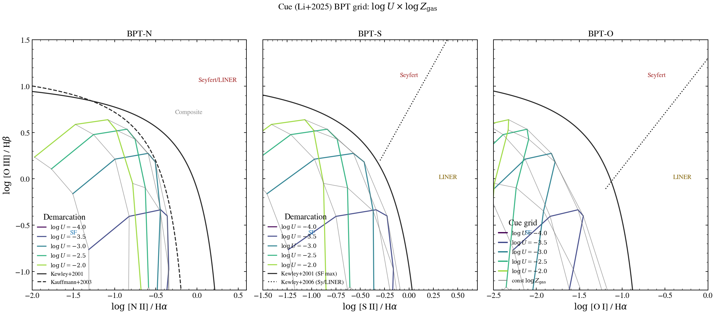
BPT Diagrams with Cue: 2D Grid in (log U, log Z_gas)

Compute three classical BPT line-ratio diagrams using the Cue emulator (Li+2025) and overplot the standard 2D nebular grid: lines of constant log U (varying gas metallicity) and lines of constant log Z_gas (varying ionization parameter). This is the canonical view in Kewley+2001/2013, Dopita+2013, and similar nebular-grid papers.

Three panels:

• BPT-N : log [O III]/Hβ vs log [N II]/Hα

• BPT-S : log [O III]/Hβ vs log [S II]/Hα

• BPT-O : log [O III]/Hβ vs log [O I]/Hα

Demarcations:

• Kewley+2001 maximum-starburst envelope (solid)

• Kauffmann+2003 empirical SF-galaxy boundary (dashed, BPT-N only)

• Kewley+2006 Seyfert/LINER divider (dotted, BPT-S and BPT-O)

Increasing log U pushes the grid up and to the left (harder ionization field, more high-ionization lines like [O III]). Increasing log Z_gas boosts collisionally-excited lines like [N II], [S II], [O I] relative to the recombination lines, pulling the grid to the right.

from pathlib import Path

import jax
import matplotlib.pyplot as plt
import numpy as np

jax.config.update("jax_enable_x64", True)

from tengri import Fixed, Parameters, SEDModel, load_ssp_data
from tengri.analysis.plotting import setup_style

setup_style()


def _find(rel: str) -> Path | None:
    for d in [Path(rel), Path("..") / rel, Path("../..") / rel, Path("../../..") / rel]:
        if d.exists():
            return d
    return None


# Cue requires a BARE-stellar SSP — wNE templates have nebular already
# baked in, which lowers Q_H below Cue's training floor. Use the
# ionizing-corrected FSPS bare grid.
SSP_PATH = _find("data/fsps_prsc_miles_chabrier.h5")
CUE_PATH = _find("data/cue_weights.npz")
if SSP_PATH is None or CUE_PATH is None:
    raise FileNotFoundError("SSP or Cue weights not found")

ssp = load_ssp_data(str(SSP_PATH))

# --- Cue parameters: 2D grid over (log U, log Z_gas) -----------------
LOGU_GRID = np.array([-4.0, -3.5, -3.0, -2.5, -2.0])
LOGZ_GRID = np.array([-1.5, -1.0, -0.5, -0.3, 0.0, 0.3])

# BPT diagnostic line wavelengths (vacuum, Angstrom)
LINES = {
    "Hβ": 4862.7,
    "[O III]": 5008.2,
    "[O I]": 6302.0,
    "Hα": 6564.6,
    "[N II]": 6585.3,
    "[S II]a": 6718.3,
    "[S II]b": 6732.7,
}
TARGETS = np.array([LINES[k] for k in ["Hβ", "[O III]", "[O I]", "Hα", "[N II]", "[S II]a", "[S II]b"]])


def _bpt_ratios(logu: float, logz: float) -> dict[str, float]:
    """Return BPT line ratios for one (log U, log Z_gas) point via Cue."""
    spec = Parameters(
        sfh_tsnorm_log_peak_sfr=Fixed(1.0),
        sfh_tsnorm_peak_lbt_gyr=Fixed(0.05),  # young burst → strong ionizing field
        sfh_tsnorm_width_gyr=Fixed(0.02),
        sfh_tsnorm_skew=Fixed(0.0),
        sfh_tsnorm_trunc=Fixed(0.5),
        met_logzsol=Fixed(logz),
        dust_tau_bc=Fixed(0.0),
        dust_tau_diff=Fixed(0.0),
        dust_slope=Fixed(-0.7),
        redshift=Fixed(0.05),
        neb_logU=Fixed(logu),
        neb_logZ_gas=Fixed(logz),
        neb_fesc=Fixed(0.0),
        nebular="cue",
        cue_weights_path=str(CUE_PATH),
    )
    model = SEDModel(spec, ssp)
    fluxes = np.asarray(model.predict_line_fluxes(spec.get_fixed_values(), target_wavelengths=TARGETS))
    f_hb, f_o3, f_o1, f_ha, f_n2, f_s2a, f_s2b = fluxes
    return {
        "log_o3_hb": np.log10(f_o3 / f_hb) if f_hb > 0 else np.nan,
        "log_n2_ha": np.log10(f_n2 / f_ha) if f_ha > 0 else np.nan,
        "log_s2_ha": np.log10((f_s2a + f_s2b) / f_ha) if f_ha > 0 else np.nan,
        "log_o1_ha": np.log10(f_o1 / f_ha) if f_ha > 0 else np.nan,
    }


# --- Build the (logU, logZ) → ratio mesh ----------------------------
mesh = np.empty((len(LOGU_GRID), len(LOGZ_GRID)), dtype=object)
for i, logu in enumerate(LOGU_GRID):
    for j, logz in enumerate(LOGZ_GRID):
        mesh[i, j] = _bpt_ratios(float(logu), float(logz))

# Stack into 2D arrays for vectorised plotting
oh = np.array([[mesh[i, j]["log_o3_hb"] for j in range(len(LOGZ_GRID))] for i in range(len(LOGU_GRID))])
nh = np.array([[mesh[i, j]["log_n2_ha"] for j in range(len(LOGZ_GRID))] for i in range(len(LOGU_GRID))])
sh = np.array([[mesh[i, j]["log_s2_ha"] for j in range(len(LOGZ_GRID))] for i in range(len(LOGU_GRID))])
oih = np.array([[mesh[i, j]["log_o1_ha"] for j in range(len(LOGZ_GRID))] for i in range(len(LOGU_GRID))])


# --- Demarcation lines ----------------------------------------------
def kewley01_n2(x):
    return 0.61 / (x - 0.47) + 1.19  # Kewley+2001 max starburst


def kauff03_n2(x):
    return 0.61 / (x - 0.05) + 1.30  # Kauffmann+2003 empirical SF


def kewley01_s2(x):
    return 0.72 / (x - 0.32) + 1.30  # Kewley+2001 SF max for [S II]


def kewley06_seyfert_s2(x):
    return 1.89 * x + 0.76  # Kewley+2006 Seyfert/LINER for [S II]


def kewley01_o1(x):
    return 0.73 / (x + 0.59) + 1.33  # Kewley+2001 SF max for [O I]


def kewley06_seyfert_o1(x):
    return 1.18 * x + 1.30  # Kewley+2006 Seyfert/LINER for [O I]


# --- Plot 1×3 BPT panels --------------------------------------------
fig, axes = plt.subplots(1, 3, figsize=(16, 7), sharey=True)


def _draw_grid(ax, x_arr, y_arr, x_label, demarcations, region_labels):
    """Draw the Cue (logU × logZ) grid plus demarcation lines on one BPT panel."""
    cmap = plt.cm.viridis
    # Lines of constant logU, varying logZ (rows)
    for i, logu in enumerate(LOGU_GRID):
        c = cmap(0.0 + 0.85 * i / max(len(LOGU_GRID) - 1, 1))
        ax.plot(x_arr[i, :], y_arr[i, :], "-", lw=1.6, color=c, alpha=0.95,
                label=rf"$\log U = {logu:.1f}$")
    # Lines of constant logZ, varying logU (columns) — drawn thinner in grey
    for j in range(len(LOGZ_GRID)):
        ax.plot(x_arr[:, j], y_arr[:, j], "-", lw=0.8, color="0.45", alpha=0.7)
    # Demarcations
    for label, xs, ys, style in demarcations:
        ax.plot(xs, ys, style, lw=1.6, color="0.15", label=label)
    # Region annotations
    for txt, xy, color in region_labels:
        ax.text(*xy, txt, fontsize=10, color=color, ha="center")
    ax.set_xlabel(x_label)
    ax.grid(False)


# BPT-N
n2_grid = np.linspace(-2.0, 0.45, 200)
demarc_n = [
    ("Kewley+2001", n2_grid[n2_grid < 0.47], kewley01_n2(n2_grid[n2_grid < 0.47]), "-"),
    ("Kauffmann+2003", n2_grid[n2_grid < 0.05], kauff03_n2(n2_grid[n2_grid < 0.05]), "--"),
]
regions_n = [
    ("SF", (-1.5, -0.6), "#1f77b4"),
    ("Composite", (-0.1, 0.7), "#888"),
    ("Seyfert/LINER", (0.25, 1.05), "#a02020"),
]
_draw_grid(axes[0], nh, oh, r"$\log\,$[N II] / H$\alpha$", demarc_n, regions_n)
axes[0].set_title("BPT-N")
axes[0].set_xlim(-2.0, 0.6)

# BPT-S
s2_grid = np.linspace(-1.5, 0.6, 200)
demarc_s = [
    ("Kewley+2001 (SF max)", s2_grid[s2_grid < 0.32], kewley01_s2(s2_grid[s2_grid < 0.32]), "-"),
    ("Kewley+2006 (Sy/LINER)", s2_grid[s2_grid > -0.3], kewley06_seyfert_s2(s2_grid[s2_grid > -0.3]), ":"),
]
regions_s = [
    ("SF", (-1.0, -0.6), "#1f77b4"),
    ("Seyfert", (0.0, 1.1), "#a02020"),
    ("LINER", (0.4, 0.0), "#806000"),
]
_draw_grid(axes[1], sh, oh, r"$\log\,$[S II] / H$\alpha$", demarc_s, regions_s)
axes[1].set_title("BPT-S")
axes[1].set_xlim(-1.5, 0.7)

# BPT-O
o1_grid = np.linspace(-2.5, 0.0, 200)
demarc_o = [
    ("Kewley+2001 (SF max)", o1_grid[o1_grid < -0.59], kewley01_o1(o1_grid[o1_grid < -0.59]), "-"),
    ("Kewley+2006 (Sy/LINER)", o1_grid[o1_grid > -1.2], kewley06_seyfert_o1(o1_grid[o1_grid > -1.2]), ":"),
]
regions_o = [
    ("SF", (-2.1, -0.6), "#1f77b4"),
    ("Seyfert", (-0.6, 1.1), "#a02020"),
    ("LINER", (-0.3, 0.0), "#806000"),
]
_draw_grid(axes[2], oih, oh, r"$\log\,$[O I] / H$\alpha$", demarc_o, regions_o)
axes[2].set_title("BPT-O")
axes[2].set_xlim(-2.5, 0.0)

axes[0].set_ylabel(r"$\log\,$[O III] / H$\beta$")
for ax in axes:
    ax.set_ylim(-1.2, 1.5)

# Per-panel legends. Each panel gets its own demarcation legend (distinct
# between BPT-N, BPT-S, BPT-O); the rightmost panel additionally lists the
# logU curves and the constant-logZ helper line.
logu_handles = [plt.Line2D([0], [0], color=plt.cm.viridis(0.85 * i / max(len(LOGU_GRID) - 1, 1)),
                            lw=2.0, label=rf"$\log U = {u:.1f}$") for i, u in enumerate(LOGU_GRID)]
logu_handles.append(plt.Line2D([0], [0], color="0.45", lw=1.0, label=r"const $\log Z_{\rm gas}$"))
axes[0].legend(loc="lower left", fontsize=9, frameon=False, title="Demarcation")
axes[1].legend(loc="lower left", fontsize=9, frameon=False, title="Demarcation")
axes[2].legend(handles=logu_handles, loc="lower left", fontsize=9, frameon=False,
               title="Cue grid")

fig.suptitle(
    r"Cue (Li+2025) BPT grid: $\log U \times \log Z_{\rm gas}$",
    fontsize=14, y=1.0,
)
fig.tight_layout()
plt.savefig("plot_bpt_cue_grid.png", dpi=150, bbox_inches="tight")
plt.show()