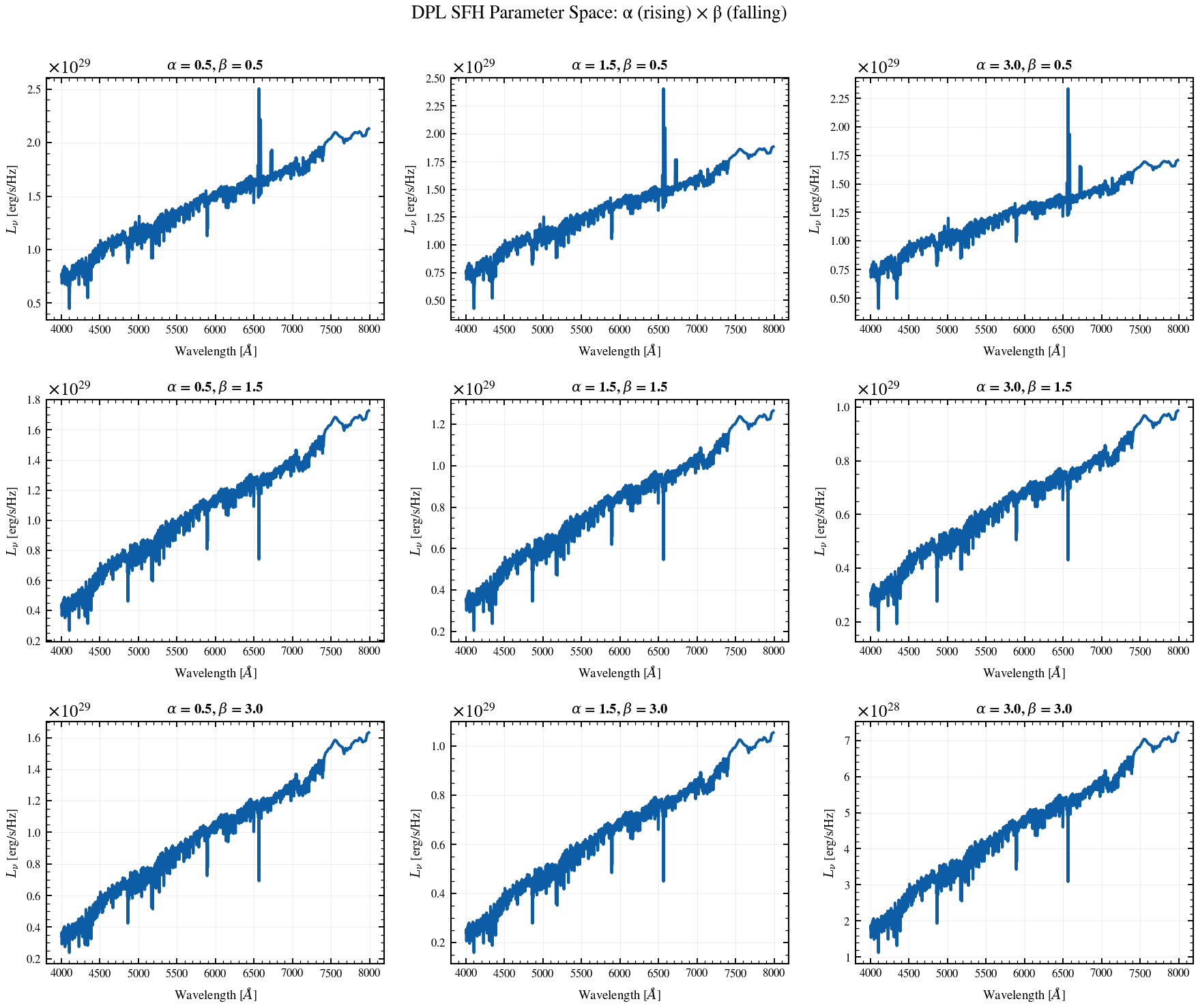
Double Power-Law SFH: 2D Parameter Grid (α × β)

Visualize a 3×3 grid of double power-law SFH shapes, sweeping the rising slope α and falling slope β to show how the parameter space controls SFH morphology.

from pathlib import Path

import jax
import matplotlib.pyplot as plt
import numpy as np

jax.config.update("jax_enable_x64", True)

from tengri import Fixed, Parameters, SEDModel, load_ssp_data
from tengri.analysis.plotting import setup_style

setup_style()


def _find_ssp():
    """Find SSP data file in standard locations."""
    name = "ssp_prsc_miles_chabrier_wNE_logGasU-3.0_logGasZ0.0.h5"
    for p in [
        Path("data") / name,
        Path("../data") / name,
        Path("../../data") / name,
        Path("../../../data") / name,
    ]:
        if p.exists():
            return str(p)
    return None


SSP_PATH = _find_ssp()
if SSP_PATH is None:
    raise FileNotFoundError("SSP data not found — skipping example")

ssp = load_ssp_data(SSP_PATH)

# Shared baseline
shared = dict(
    sfh_dpl_tau_gyr=Fixed(3.0),
    sfh_dpl_log_peak_sfr=Fixed(1.0),
    met_logzsol=Fixed(-0.3),
    dust_tau_bc=Fixed(0.3),
    dust_tau_diff=Fixed(0.2),
    dust_slope=Fixed(-0.7),
    redshift=Fixed(0.1),
)

# Grid: alpha (rising slope) and beta (falling slope)
alphas = [0.5, 1.5, 3.0]
betas = [0.5, 1.5, 3.0]

fig, axes = plt.subplots(3, 3, figsize=(12, 10))
fig.suptitle("DPL SFH Parameter Space: α (rising) × β (falling)", fontsize=13, y=0.995)

for i, beta in enumerate(betas):
    for j, alpha in enumerate(alphas):
        ax = axes[i, j]

        spec = Parameters(
            mean_sfh_type="dpl",
            sfh_dpl_alpha=Fixed(alpha),
            sfh_dpl_beta=Fixed(beta),
            **shared,
        )
        model = SEDModel(spec, ssp)

        params_eval = {k: float(v.value) for k, v in shared.items()}
        params_eval.update({"sfh_dpl_alpha": alpha, "sfh_dpl_beta": beta})

        sed = model.predict_rest_sed(params_eval).sed

        # Optical region
        wave_opt = np.array(ssp.ssp_wave)
        mask = (wave_opt > 4000) & (wave_opt < 8000)

        ax.plot(
            wave_opt[mask],
            np.array(sed[mask]),
            "C0-",
            lw=2.0,
        )
        ax.set_xlabel(r"Wavelength [$\AA$]", fontsize=9)
        ax.set_ylabel(r"$L_\nu$ [erg/s/Hz]", fontsize=9)
        ax.set_title(rf"$\alpha$ = {alpha}, $\beta$ = {beta}", fontsize=10, fontweight="bold")
        ax.grid(True, alpha=0.2)
        ax.tick_params(labelsize=8)

fig.tight_layout()
plt.savefig("plot_dpl_alpha_beta_grid.png", dpi=150, bbox_inches="tight")
plt.show()