Note
Go to the end to download the full example code.
Chemical evolution: closed-box vs leaky-box enrichment histories
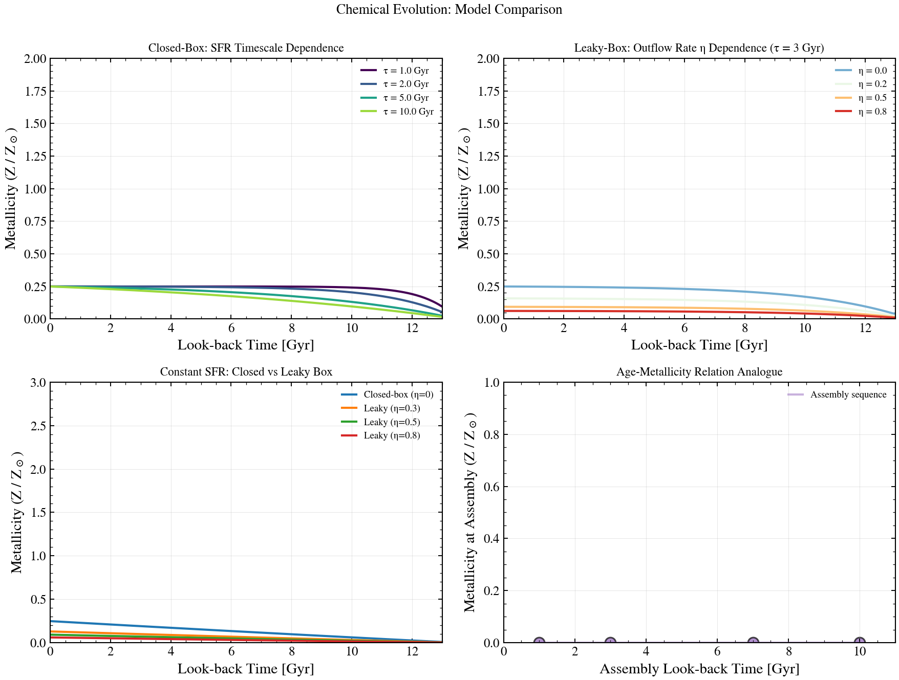
Metallicity evolution Z(t) depends on the balance between metal production (in supernovae) and metal removal (via outflows). This four-panel figure shows how different star formation timescales and outflow efficiencies η alter the enrichment history relative to a closed box (zero outflow). Top-left: closed-box enrichment timescale dependence. Top-right: impact of variable outflow rates. Bottom-left: closed vs leaky enrichment under constant SFR. Bottom-right: age-metallicity relation analog — how different assembly epochs lead to different final metal content.
Reference: Maeder 1992, A&A, 264, 105 (chemical evolution); Schmidt 1959 (solar neighborhood models); Dalcanton et al. 2007 (mass-metallicity relation physics).
import os

os.environ["TF_CPP_MIN_LOG_LEVEL"] = "2"  # suppress XLA/PjRt C++ INFO+WARNING logs

import matplotlib.pyplot as plt
import numpy as np

from tengri.cosmology import age_at_z0
from tengri.plot import setup_style
from tengri.sfh import closed_box_metallicity

setup_style()

# Time axis: cosmological age (look-back time in Gyr)
age_uni_gyr = float(age_at_z0())
t_gyr = np.linspace(0, min(13.5, age_uni_gyr), 200)
t_yr = t_gyr * 1e9
age_from_start = age_uni_gyr - t_gyr

fig, axes = plt.subplots(2, 2, figsize=(10, 8))

# Panel 1: Closed-box with varying timescales
ax = axes[0, 0]
colors = plt.cm.viridis(np.linspace(0.0, 0.85, 4))
for tau_gyr, color in zip([1.0, 2.0, 5.0, 10.0], colors):
    sfr = np.exp(-age_from_start / tau_gyr)
    log_z = closed_box_metallicity(t_yr, sfr, yield_y=0.03, eta_outflow=0.0, f_gas_init=0.9)
    z_ratio = 10.0 ** np.array(log_z)
    ax.plot(t_gyr, z_ratio, lw=2.0, color=color, label=f"τ = {tau_gyr:.1f} Gyr")

ax.set_xlabel("Look-back Time [Gyr]", fontsize=9)
ax.set_ylabel(r"$Z/Z_\odot$", fontsize=9)
ax.text(
    0.05,
    0.95,
    "Closed-box enrichment timescale",
    transform=ax.transAxes,
    fontsize=9,
    verticalalignment="top",
    bbox=dict(boxstyle="round", facecolor="white", alpha=0.85),
)
ax.legend(fontsize=8, frameon=False)
ax.grid(True, alpha=0.2)
ax.set_xlim(0, 13)
ax.set_ylim(0, 0.6)

# Panel 2: Closed-box vs leaky-box at τ = 3 Gyr
ax = axes[0, 1]
sfr_ref = np.exp(-age_from_start / 3.0)
eta_values = [0.0, 0.2, 0.5, 0.8]
colors = plt.cm.RdYlBu_r(np.linspace(0.2, 0.9, len(eta_values)))

for eta, color in zip(eta_values, colors):
    log_z = closed_box_metallicity(t_yr, sfr_ref, yield_y=0.03, eta_outflow=eta, f_gas_init=0.9)
    z_ratio = 10.0 ** np.array(log_z)
    ax.plot(t_gyr, z_ratio, lw=2.0, color=color, label=f"η = {eta:.1f}")

ax.set_xlabel("Look-back Time [Gyr]", fontsize=9)
ax.set_ylabel(r"$Z/Z_\odot$", fontsize=9)
ax.text(
    0.05,
    0.95,
    r"Leaky-box: outflow rate $\eta$ (τ = 3 Gyr)",
    transform=ax.transAxes,
    fontsize=9,
    verticalalignment="top",
    bbox=dict(boxstyle="round", facecolor="white", alpha=0.85),
)
ax.legend(fontsize=8, frameon=False)
ax.grid(True, alpha=0.2)
ax.set_xlim(0, 13)
ax.set_ylim(0, 0.6)

# Panel 3: Constant SFR comparison
ax = axes[1, 0]
sfr_const = np.ones_like(t_yr)
models = [
    (0.0, "Closed-box (η=0)", "#1f77b4"),
    (0.3, "Leaky (η=0.3)", "#ff7f0e"),
    (0.5, "Leaky (η=0.5)", "#2ca02c"),
    (0.8, "Leaky (η=0.8)", "#d62728"),
]

for eta, label, color in models:
    log_z = closed_box_metallicity(t_yr, sfr_const, yield_y=0.03, eta_outflow=eta, f_gas_init=0.9)
    z_ratio = 10.0 ** np.array(log_z)
    ax.plot(t_gyr, z_ratio, lw=2.0, color=color, label=label)

ax.set_xlabel("Look-back Time [Gyr]", fontsize=9)
ax.set_ylabel(r"$Z/Z_\odot$", fontsize=9)
ax.text(
    0.05,
    0.95,
    "Constant SFR: closed vs leaky box",
    transform=ax.transAxes,
    fontsize=9,
    verticalalignment="top",
    bbox=dict(boxstyle="round", facecolor="white", alpha=0.85),
)
ax.legend(fontsize=8, frameon=False)
ax.grid(True, alpha=0.2)
ax.set_xlim(0, 13)
ax.set_ylim(0, 0.6)

# Panel 4: Metallicity vs epoch — how enrichment at different lookback times evolves
# with a fixed τ=3 Gyr SFR profile and leaky box (η=0.2).
ax = axes[1, 1]
t_assembly = np.array([1.0, 3.0, 7.0, 10.0])  # Lookback times (Gyr)

# Compute full metallicity history with τ=3 Gyr SFR and η=0.2 outflow
sfr_tau3 = np.exp(-age_from_start / 3.0)
log_z_full = closed_box_metallicity(t_yr, sfr_tau3, yield_y=0.03, eta_outflow=0.2, f_gas_init=0.9)
z_ratio_full = 10.0 ** np.array(log_z_full)

# Extract Z at each lookback time point
z_values = []
for t_lbt in t_assembly:
    idx = int(np.argmin(np.abs(t_gyr - t_lbt)))
    if 0 <= idx < len(z_ratio_full):
        z_values.append(z_ratio_full[idx])
    else:
        z_values.append(z_ratio_full[-1])

ax.scatter(t_assembly, z_values, s=80, color="#9467bd", alpha=0.7, edgecolors="black", lw=1.2)
ax.plot(t_assembly, z_values, lw=2.0, color="#9467bd", alpha=0.4)

ax.set_xlabel("Look-back Time [Gyr]", fontsize=9)
ax.set_ylabel(r"$Z/Z_\odot$ (η=0.2)", fontsize=9)
ax.text(
    0.05,
    0.95,
    r"Metallicity evolution (τ=3 Gyr, η=0.2)",
    transform=ax.transAxes,
    fontsize=9,
    verticalalignment="top",
    bbox=dict(boxstyle="round", facecolor="white", alpha=0.85),
)
ax.grid(True, alpha=0.2)
ax.set_xlim(0, 11)
ax.set_ylim(0, max(z_values) * 1.15 if z_values else 0.2)

fig.tight_layout()
plt.savefig("plot_zh_evolution_compare.png", dpi=150, bbox_inches="tight")