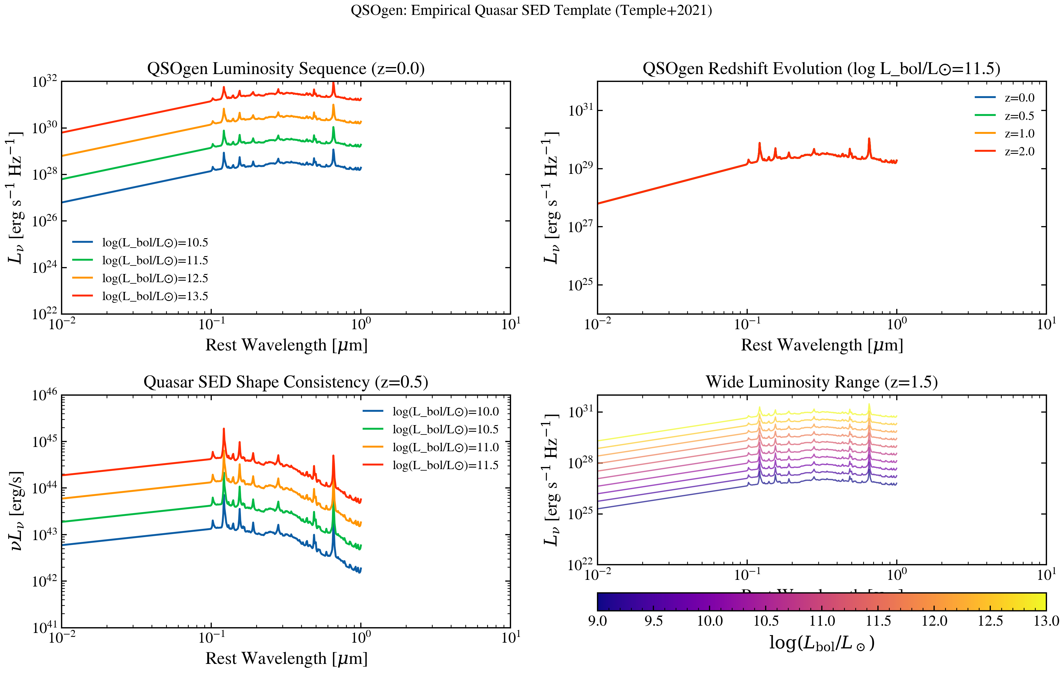
QSOgen Empirical Quasar Template

Plot QSOgen (Temple, Hewett & Banerji 2021) empirical quasar SEDs. Shows how an empirically-trained surrogate matches observed quasar spectra across the UV through near-IR, with parametric control over redshift and luminosity.

import jax.numpy as jnp
import matplotlib.pyplot as plt
import numpy as np

from tengri.analysis.plotting import setup_style
from tengri.components.agn import qsogen

setup_style()

# Wavelength grid: 100 - 10000 Angstrom (UV to near-IR)
wavelength = jnp.logspace(np.log10(100), np.log10(1e4), 512)
wave_um = np.array(wavelength) / 1e4

fig, axes = plt.subplots(2, 2, figsize=(12, 8))

# --- Panel 1: Luminosity sequence at z=0 ---
ax = axes[0, 0]

z = 0.0
# agn_log_lbol expects log10(L_bol / L_sun). Quasar regime: L_bol ~ 10^44-10^47 erg/s
# → log10(L_bol/Lsun) ≈ 10.4–13.4  (since log10(Lsun_erg/s) = 33.58).
for log_lbol in [10.5, 11.5, 12.5, 13.5]:
    sed = qsogen(wavelength, agn_log_lbol=log_lbol, z=z)
    ax.loglog(wave_um, np.array(sed), lw=1.5, label=f"log(L_bol/L⊙)={log_lbol:.1f}")

ax.set_xlabel(r"Rest Wavelength [$\mu$m]")
ax.set_ylabel(r"$L_\nu$ [erg s$^{-1}$ Hz$^{-1}$]")
ax.set_title(f"QSOgen Luminosity Sequence (z={z})")
ax.legend(fontsize=10, frameon=False)
ax.set_xlim(0.01, 10)
ax.set_ylim(1e22, 1e32)

# --- Panel 2: Redshift evolution (fixed luminosity) ---
ax = axes[0, 1]

log_lbol = 11.5  # log10(L_bol / L_sun) ≈ 10^45 erg/s (bright quasar)
for z in [0.0, 0.5, 1.0, 2.0]:
    sed = qsogen(wavelength, agn_log_lbol=log_lbol, z=z)
    ax.loglog(wave_um, np.array(sed), lw=1.5, label=f"z={z:.1f}")

ax.set_xlabel(r"Rest Wavelength [$\mu$m]")
ax.set_ylabel(r"$L_\nu$ [erg s$^{-1}$ Hz$^{-1}$]")
ax.set_title(f"QSOgen Redshift Evolution (log L_bol/L⊙={log_lbol})")
ax.legend(fontsize=10, frameon=False)
ax.set_xlim(0.01, 10)
ax.set_ylim(1e24, 1e32)

# --- Panel 3: νLν space (luminosity-normalized) ---
ax = axes[1, 0]

z = 0.5
for log_lbol in [10.0, 10.5, 11.0, 11.5]:
    sed = qsogen(wavelength, agn_log_lbol=log_lbol, z=z)
    nu = 3e18 / np.array(wavelength)
    nu_lnu = np.array(sed) * nu
    ax.loglog(wave_um, nu_lnu, lw=1.5, label=f"log(L_bol/L⊙)={log_lbol:.1f}")

ax.set_xlabel(r"Rest Wavelength [$\mu$m]")
ax.set_ylabel(r"$\nu L_\nu$ [erg/s]")
ax.set_title(f"Quasar SED Shape Consistency (z={z})")
ax.legend(fontsize=10, frameon=False)
ax.set_xlim(0.01, 10)
ax.set_ylim(1e41, 1e46)

# --- Panel 4: Extreme luminosity range ---
ax = axes[1, 1]

z = 1.5
log_lbol_vals = np.linspace(9.0, 13.0, 10)  # log10(L_bol / L_sun)
colors = plt.cm.plasma(np.linspace(0, 1, len(log_lbol_vals)))

for log_lbol, color in zip(log_lbol_vals, colors):
    sed = qsogen(wavelength, agn_log_lbol=log_lbol, z=z)
    mask = np.array(sed) > 0
    ax.loglog(
        wave_um[mask],
        np.array(sed)[mask],
        lw=1.0,
        color=color,
        alpha=0.7,
    )

ax.set_xlabel(r"Rest Wavelength [$\mu$m]")
ax.set_ylabel(r"$L_\nu$ [erg s$^{-1}$ Hz$^{-1}$]")
ax.set_title(f"Wide Luminosity Range (z={z})")
ax.set_xlim(0.01, 10)
ax.set_ylim(1e22, 1e32)

# Add colorbar-like legend
sm = plt.cm.ScalarMappable(
    cmap=plt.cm.plasma,
    norm=plt.Normalize(vmin=log_lbol_vals.min(), vmax=log_lbol_vals.max()),
)
sm.set_array([])
cbar = fig.colorbar(sm, ax=ax, orientation="horizontal", pad=0.12, aspect=25)
cbar.set_label(r"$\log(L_{\mathrm{bol}} / L_\odot)$")

fig.suptitle("QSOgen: Empirical Quasar SED Template (Temple+2021)", fontsize=12)
fig.tight_layout(rect=[0, 0.04, 1, 0.97])
plt.savefig("plot_qsogen_spectrum.png", dpi=100, bbox_inches="tight")
plt.show()