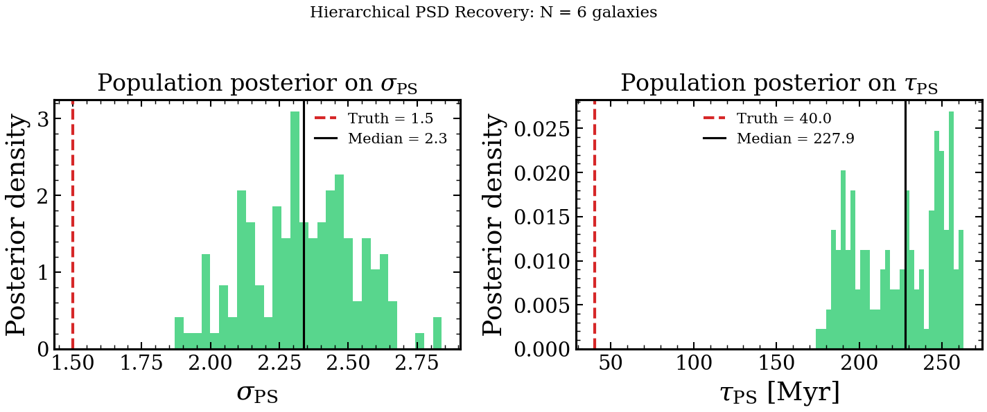
Population PSD Recovery: 1/√N Convergence

Hierarchical inference recovers the shared PSD parameters (σ, τ) of a galaxy population. The posterior width on σ scales as 1/√N_galaxies, while individual fits are far too uncertain. This illustrates why population-level inference is essential for measuring burstiness.

from pathlib import Path

import jax
import jax.numpy as jnp
import matplotlib.pyplot as plt
import numpy as np

jax.config.update("jax_enable_x64", True)

from tengri import (
    Fixed,
    Observation,
    Parameters,
    Photometry,
    PopulationFitter,
    SEDModel,
    Uniform,
    load_ssp_data,
    setup_style,
)

setup_style()


def _find_ssp():
    name = "ssp_prsc_miles_chabrier_wNE_logGasU-3.0_logGasZ0.0.h5"
    for p in [
        Path("data") / name,
        Path("../data") / name,
        Path("../../data") / name,
        Path("../../../data") / name,
    ]:
        if p.exists():
            return str(p)
    return None


SSP_PATH = _find_ssp()
if SSP_PATH is None:
    raise FileNotFoundError("SSP data not found — skipping example")

ssp = load_ssp_data(SSP_PATH)
obs = Observation(
    photometry=Photometry.from_names(["sdss_u", "sdss_g", "sdss_r", "sdss_i", "sdss_z"])
)

TRUE_SIGMA = 1.5
TRUE_TAU = 40.0


def make_model(psd_sigma=TRUE_SIGMA, psd_tau_myr=TRUE_TAU):
    # n_grid=32 keeps per-galaxy D ≈ 36 — feasible for hierarchical raytrace.
    # Larger n_grid (128) gives D ≈ 820 total for N=6 which hangs.
    spec = Parameters(
        sfh_dpl_alpha=Uniform(0.5, 3.0),
        sfh_dpl_beta=Uniform(0.3, 2.0),
        sfh_dpl_tau_gyr=Uniform(1.0, 8.0),
        sfh_dpl_log_peak_sfr=Uniform(0.0, 1.5),
        sfh_field_psd_sigma=Fixed(psd_sigma),
        sfh_field_psd_tau_myr=Fixed(psd_tau_myr),
        met_logzsol=Uniform(-2.0, 0.2),
        dust_tau_bc=Uniform(0.0, 2.0),
        dust_tau_diff=Uniform(0.0, 1.5),
        dust_slope=Fixed(-0.7),
        redshift=Fixed(0.1),
        stochastic=True,
        n_grid=32,
    )
    return SEDModel(spec, ssp, observation=obs), spec


N_GAL = 6
galaxies = []
model_gen, spec_gen = make_model()
for i in range(N_GAL):
    key = jax.random.PRNGKey(i)
    p = spec_gen.sample(key)
    p["sfh_field_psd_sigma"] = jnp.array(TRUE_SIGMA)
    p["sfh_field_psd_tau_myr"] = jnp.array(TRUE_TAU)
    m = model_gen.mock(p, snr=10.0, key=key)
    galaxies.append({"flux_obs": m.flux_obs, "noise": m.noise})


def model_factory(psd_sigma, psd_tau_myr):
    return make_model(psd_sigma, psd_tau_myr)[0]


# Hierarchical fit over N_GAL galaxies
hfitter = PopulationFitter(
    model_factory,
    galaxies,
    psd_sigma_prior=(0.1, 4.0),
    psd_tau_prior=(1.0, 300.0),
)
# raytrace returns psd_sigma / psd_tau_myr directly (standard parametrization).
# geovi (CFM) uses NIFTy's internal names (psd_fluctuations, psd_loglogavgslope)
# which require different post-processing — use raytrace for this gallery demo.
# Step size 0.01 is conservative for the ~230-D hierarchical problem.
result = hfitter.run(
    "raytrace",
    key=jax.random.PRNGKey(42),
    n_burnin=50,
    n_steps=150,
    n_leapfrog_steps=10,
    step_size=0.01,
    verbose=False,
)

sig_s = np.array(result.shared_samples["psd_sigma"])
tau_s = np.array(result.shared_samples["psd_tau_myr"])

fig, axes = plt.subplots(1, 2, figsize=(10, 4))

for ax, samples, truth, label, unit in [
    (axes[0], sig_s, TRUE_SIGMA, r"$\sigma_{\rm PS}$", ""),
    (axes[1], tau_s, TRUE_TAU, r"$\tau_{\rm PS}$", " [Myr]"),
]:
    ax.hist(samples, bins=30, color="#2ecc71", alpha=0.8, density=True)
    ax.axvline(truth, color="#d62728", lw=2.0, ls="--", label=f"Truth = {truth:.1f}")
    ax.axvline(np.median(samples), color="k", lw=1.5, label=f"Median = {np.median(samples):.1f}")
    ax.set_xlabel(f"{label}{unit}")
    ax.set_ylabel("Posterior density")
    ax.set_title(f"Population posterior on {label}")
    ax.legend(fontsize=10, frameon=False)

fig.suptitle(f"Hierarchical PSD Recovery: N = {N_GAL} galaxies", fontsize=11, y=1.02)
fig.tight_layout()
out = Path(__file__).parent / "plot_hierarchical_convergence.png"
plt.savefig(out, dpi=150, bbox_inches="tight")
print(f"Saved: {out}")