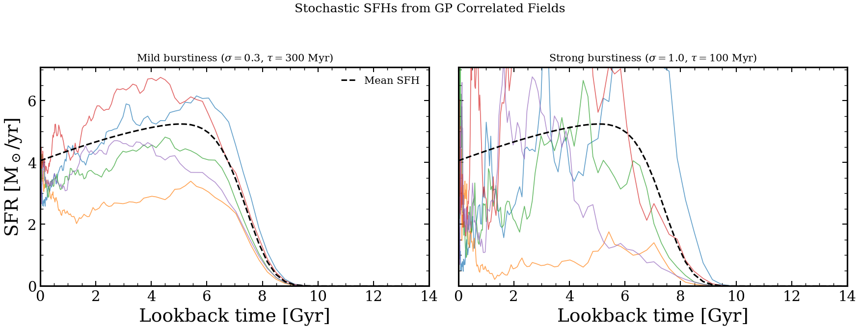
Stochastic SFH from GP Correlated Fields

Generate stochastic star formation histories using the Fourier-space GP correlated field model. The DRW (damped random walk) PSD governs the burstiness: larger sigma means more variance, shorter tau means more rapid fluctuations.

import jax
import jax.numpy as jnp
import matplotlib.pyplot as plt
import numpy as np

from tengri import (
    compute_sqrt_power_drw,
    generate_gp_fourier,
    make_log_age_grid,
    tsnorm,
)
from tengri.analysis.plotting import setup_style

setup_style()


# --- Grid setup ---
n_grid = 256
log_age_grid = make_log_age_grid(n_grid)
d_log_age = float(log_age_grid[1] - log_age_grid[0])
t_lookback = 10.0**log_age_grid
t_gyr = np.array(t_lookback) / 1e9

# --- Smooth mean SFH ---
mean_sfr = tsnorm(t_lookback, log_peak_sfr=1.0, peak_lbt=6e9, width=2e9, skew=0.5, trunc=3.0)

# --- Generate GP realizations at two different PSD settings ---
fig, axes = plt.subplots(1, 2, figsize=(12, 4.5), sharey=True)
configs = [
    {"sigma": 0.3, "tau_myr": 300, "title": r"Mild burstiness ($\sigma=0.3$, $\tau=300$ Myr)"},
    {"sigma": 1.0, "tau_myr": 100, "title": r"Strong burstiness ($\sigma=1.0$, $\tau=100$ Myr)"},
]

for ax, cfg in zip(axes, configs):
    sqrt_p = compute_sqrt_power_drw(n_grid, d_log_age, cfg["sigma"], cfg["tau_myr"] * 1e6)
    ax.plot(t_gyr, np.array(mean_sfr), "k--", lw=1.5, label="Mean SFH", zorder=5)

    for i in range(5):
        key = jax.random.PRNGKey(i)
        gp = generate_gp_fourier(key, sqrt_p, n_grid)
        # Full SFH = mean * exp(GP - variance/2) for lognormal correction
        variance = float(jnp.var(gp))
        sfr = mean_sfr * jnp.exp(gp - variance / 2.0)
        ax.plot(t_gyr, np.array(sfr), lw=0.8, alpha=0.7)

    ax.set_xlabel("Lookback time [Gyr]")
    ax.set_title(cfg["title"], fontsize=10)
    ax.set_xlim(0, 14)
    ax.set_ylim(0, None)

axes[0].set_ylabel("SFR [M$_\\odot$/yr]")
axes[0].legend(fontsize=10, frameon=False)
fig.suptitle("Stochastic SFHs from GP Correlated Fields", fontsize=12, y=1.02)
fig.tight_layout()
plt.savefig("plot_stochastic_sfh.png", dpi=150, bbox_inches="tight")
plt.show()