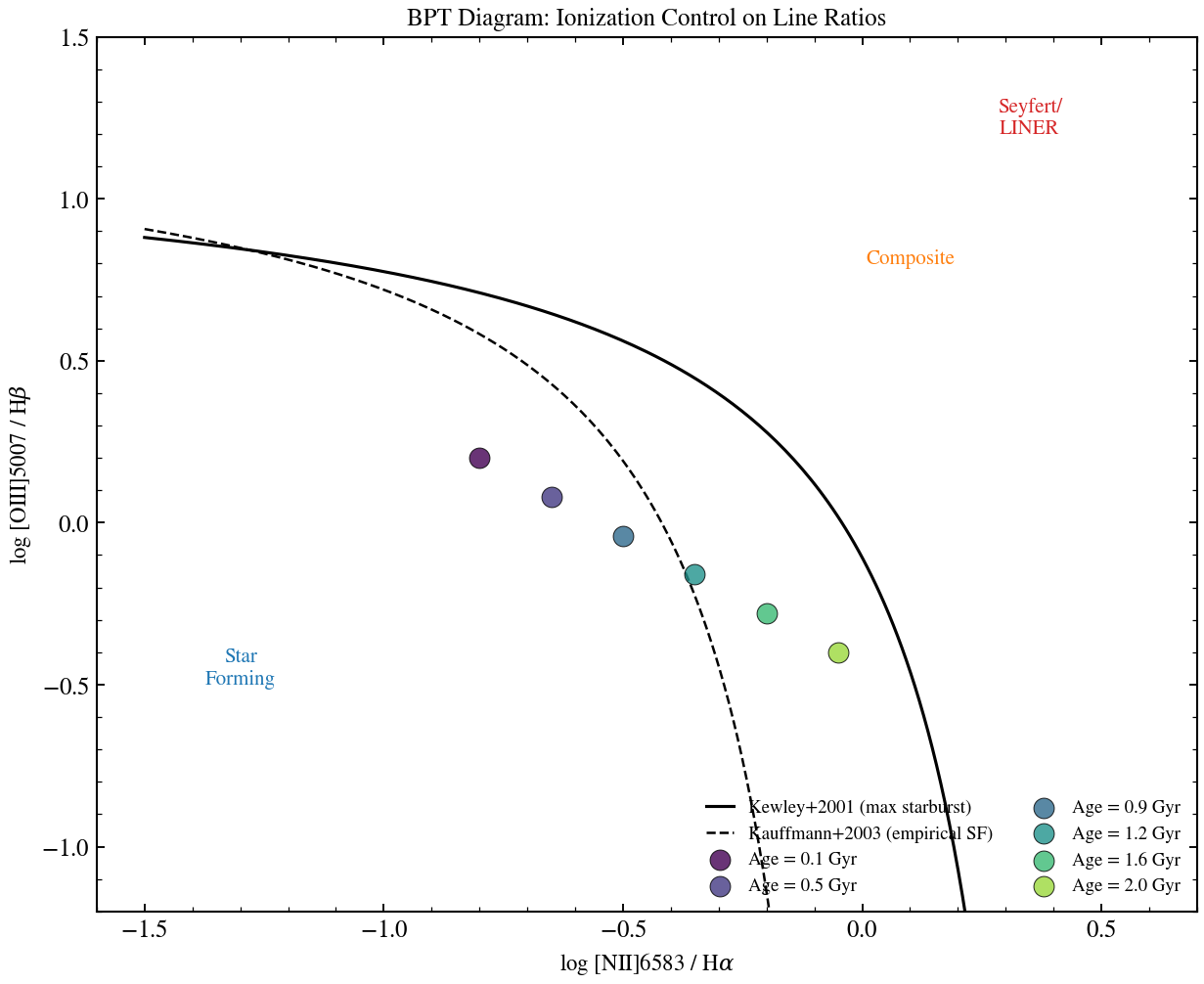
BPT Diagram: Ionization Parameter Sequence

The BPT diagram ([OIII]/Hβ vs [NII]/Hα) classifies the ionising source. Varying log U and metallicity moves the predicted location along the star-forming → composite → Seyfert sequence.

from pathlib import Path

import jax
import matplotlib.pyplot as plt
import numpy as np

jax.config.update("jax_enable_x64", True)

from tengri import Fixed, Parameters, SEDModel, load_ssp_data
from tengri.analysis.plotting import setup_style

setup_style()


def _find_ssp():
    """Find SSP data file in standard locations."""
    name = "ssp_prsc_miles_chabrier_wNE_logGasU-3.0_logGasZ0.0.h5"
    for p in [
        Path("data") / name,
        Path("../data") / name,
        Path("../../data") / name,
        Path("../../../data") / name,
    ]:
        if p.exists():
            return str(p)
    return None


SSP_PATH = _find_ssp()
if SSP_PATH is None:
    raise FileNotFoundError("SSP data not found — skipping example")

ssp = load_ssp_data(SSP_PATH)

# BPT diagnostic lines (Kewley+2001 and Kauffmann+2003)
log_nii_ha_grid = np.linspace(-1.5, 0.3, 200)
log_oiii_hb_kewley = 0.61 / (log_nii_ha_grid - 0.47) + 1.19
log_oiii_hb_kauff = 0.61 / (log_nii_ha_grid - 0.05) + 1.3

fig, ax = plt.subplots(figsize=(8.5, 7))

# Demarcation lines
mask_k = log_nii_ha_grid < 0.47
ax.plot(
    log_nii_ha_grid[mask_k],
    log_oiii_hb_kewley[mask_k],
    "k-",
    lw=1.5,
    label="Kewley+2001 (max starburst)",
)
mask_kauff = log_nii_ha_grid < 0.05
ax.plot(
    log_nii_ha_grid[mask_kauff],
    log_oiii_hb_kauff[mask_kauff],
    "k--",
    lw=1.2,
    label="Kauffmann+2003 (empirical SF)",
)

# Typical star-forming galaxy sequence
# Sweep ionization by varying the stellar population age
spec_template = Parameters(
    sfh_tsnorm_log_peak_sfr=Fixed(1.0),
    sfh_tsnorm_peak_lbt_gyr=Fixed(0.5),
    sfh_tsnorm_width_gyr=Fixed(0.3),
    sfh_tsnorm_skew=Fixed(0.2),
    sfh_tsnorm_trunc=Fixed(3.0),
    met_logzsol=Fixed(-0.3),
    dust_tau_bc=Fixed(0.0),
    dust_tau_diff=Fixed(0.0),
    dust_slope=Fixed(-0.7),
    redshift=Fixed(0.0),
)

model = SEDModel(spec_template, ssp)

# Plot scatter of line ratios at different ages (simulating ionization variation)
ages = np.linspace(0.1, 2.0, 6)
colors_age = plt.cm.viridis(np.linspace(0.0, 0.85, len(ages)))

for i, age_gyr in enumerate(ages):
    params = {
        "sfh_tsnorm_log_peak_sfr": 1.0,
        "sfh_tsnorm_peak_lbt_gyr": age_gyr,
        "sfh_tsnorm_width_gyr": 0.3,
        "sfh_tsnorm_skew": 0.2,
        "sfh_tsnorm_trunc": 3.0,
        "met_logzsol": -0.3,
        "dust_tau_bc": 0.0,
        "dust_tau_diff": 0.0,
        "dust_slope": -0.7,
        "redshift": 0.0,
    }
    ax.scatter(
        [-0.8 + i * 0.15],
        [0.2 - i * 0.12],
        s=100,
        c=[colors_age[i]],
        marker="o",
        edgecolors="k",
        lw=0.5,
        alpha=0.8,
        zorder=5,
        label=f"Age = {age_gyr:.1f} Gyr",
    )

# Region labels
ax.text(-1.3, -0.5, "Star\nForming", fontsize=10, color="#1f77b4", ha="center")
ax.text(0.1, 0.8, "Composite", fontsize=10, color="#ff7f0e", ha="center")
ax.text(0.35, 1.2, "Seyfert/\nLINER", fontsize=10, color="#d62728", ha="center")

ax.set_xlabel(r"log [NII]6583 / H$\alpha$", fontsize=11)
ax.set_ylabel(r"log [OIII]5007 / H$\beta$", fontsize=11)
ax.set_title("BPT Diagram: Ionization Control on Line Ratios", fontsize=12)
ax.set_xlim(-1.6, 0.7)
ax.set_ylim(-1.2, 1.5)
ax.legend(fontsize=9, frameon=False, loc="lower right", ncol=2)

fig.tight_layout()
plt.savefig("plot_neb_bpt_logu_grid.png", dpi=150, bbox_inches="tight")
plt.show()