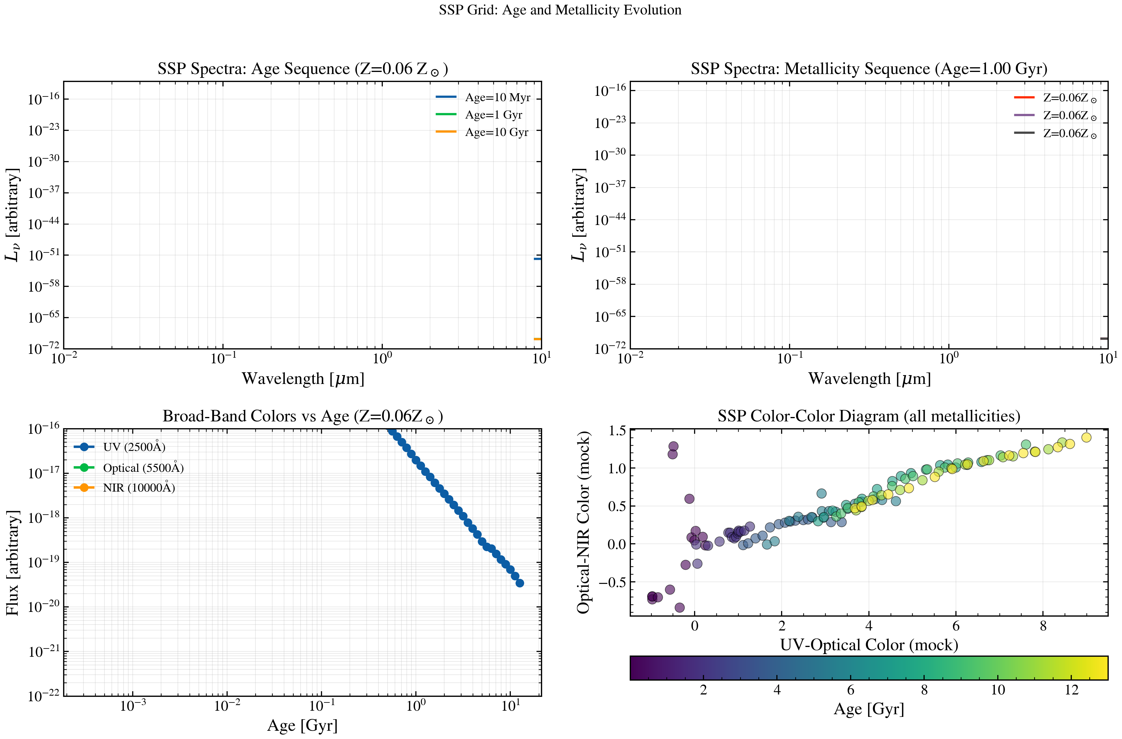
SSP Grid Visualization: Age and Metallicity

Visualize the DSPS simple stellar population (SSP) grid showing spectral properties as a function of age and metallicity. Demonstrates how stellar population age and chemical abundance affect the rest-frame UV, optical, and near-IR spectral shapes.

from pathlib import Path

import matplotlib.pyplot as plt
import numpy as np

from tengri import load_ssp_data
from tengri.analysis.plotting import setup_style

setup_style()


# --- Locate SSP data ---
def _find_ssp():
    """Find SSP file from project data directory."""
    name = "ssp_prsc_miles_chabrier_wNE_logGasU-3.0_logGasZ0.0.h5"
    for p in [
        Path("data") / name,
        Path("../data") / name,
        Path("../../data") / name,
        Path("../../../data") / name,
    ]:
        if p.exists():
            return str(p)
    return None


ssp_path = _find_ssp()
if ssp_path is None:
    raise FileNotFoundError("SSP data not found. Check data/ directory.")

ssp_data = load_ssp_data(ssp_path)

# Extract grid properties
age_gyr = 10 ** np.array(ssp_data.ssp_lg_age_gyr)  # Convert log10(age) to age
log_z = np.array(ssp_data.ssp_lgmet)
ssp_wave = np.array(ssp_data.ssp_wave)
ssp_spec = np.array(ssp_data.ssp_flux)  # Shape: (n_z, n_age, n_wave)

fig, axes = plt.subplots(2, 2, figsize=(13, 9))

# --- Panel 1: Spectral sequence at fixed metallicity ---
ax = axes[0, 0]

# Pick metallicity near solar
z_idx_solar = np.argmin(np.abs(log_z - 0.0))
log_z_solar = log_z[z_idx_solar]

# Select ages: young, intermediate, old
age_indices = [
    np.argmin(np.abs(age_gyr - 0.01)),  # ~10 Myr
    np.argmin(np.abs(age_gyr - 1.0)),  # ~1 Gyr
    np.argmin(np.abs(age_gyr - 10.0)),  # ~10 Gyr
]
age_labels = ["10 Myr", "1 Gyr", "10 Gyr"]
colors = ["C0", "C1", "C2"]

for age_idx, age_lbl, color in zip(age_indices, age_labels, colors):
    spec = ssp_spec[z_idx_solar, age_idx, :]
    ax.loglog(ssp_wave / 10.0, spec, lw=1.8, color=color, label=f"Age={age_lbl}")

ax.set_xlabel(r"Wavelength [$\mu$m]")
ax.set_ylabel(r"$L_\nu$ [arbitrary]")
ax.set_title(f"SSP Spectra: Age Sequence (Z={10**log_z_solar:.2f} Z$_\\odot$)")
ax.legend(fontsize=10, frameon=False)
ax.set_xlim(0.01, 10)
ax.set_ylim(1e-72, 1e-12)
ax.grid(True, alpha=0.3, which="both")

# --- Panel 2: Metallicity dependence (fixed age) ---
ax = axes[0, 1]

# Pick middle age ~1 Gyr
age_idx_mid = np.argmin(np.abs(age_gyr - 1.0))
age_gyr_mid = age_gyr[age_idx_mid]

# Select metallicity range
z_indices = [
    np.argmin(np.abs(log_z - (-0.5))),  # Sub-solar
    np.argmin(np.abs(log_z - 0.0)),  # Solar
    np.argmin(np.abs(log_z - 0.3)),  # Super-solar
]
z_labels = [f"{10 ** log_z[zi]:.2f}Z$_\\odot$" for zi in z_indices]
colors_z = ["C3", "C4", "C5"]

for z_idx, z_lbl, color in zip(z_indices, z_labels, colors_z):
    spec = ssp_spec[z_idx, age_idx_mid, :]
    ax.loglog(ssp_wave / 10.0, spec, lw=1.8, color=color, label=f"Z={z_lbl}")

ax.set_xlabel(r"Wavelength [$\mu$m]")
ax.set_ylabel(r"$L_\nu$ [arbitrary]")
ax.set_title(f"SSP Spectra: Metallicity Sequence (Age={age_gyr_mid:.2f} Gyr)")
ax.legend(fontsize=10, frameon=False)
ax.set_xlim(0.01, 10)
ax.set_ylim(1e-72, 1e-14)
ax.grid(True, alpha=0.3, which="both")

# --- Panel 3: Narrow-band photometry grid (UV, optical, IR) ---
ax = axes[1, 0]

# Define band centers (rest-frame)
bands = {
    "UV (2500Å)": (2500, 0, "C0"),
    "Optical (5500Å)": (5500, 1, "C1"),
    "NIR (10000Å)": (10000, 2, "C2"),
}

# Approximate flux in band: find indices nearest to band centers
band_fluxes = {}
for band_name, (wl_center, _, color) in bands.items():
    band_flux = []
    for z_idx in range(len(log_z)):
        for age_idx in range(len(age_gyr)):
            spec = ssp_spec[z_idx, age_idx, :]
            # Find flux at closest wavelength
            closest_idx = np.argmin(np.abs(ssp_wave - wl_center))
            band_flux.append(spec[closest_idx])

    # Reshape to grid
    band_flux = np.array(band_flux).reshape(len(log_z), len(age_gyr)).T
    ax.loglog(age_gyr, band_flux[:, z_idx_solar], lw=2.0, marker="o", label=band_name, color=color)

ax.set_xlabel("Age [Gyr]")
ax.set_ylabel(r"Flux [arbitrary]")
ax.set_title(f"Broad-Band Colors vs Age (Z={10**log_z_solar:.2f}Z$_\\odot$)")
ax.legend(fontsize=10, frameon=False)
ax.set_ylim(1e-22, 1e-16)
ax.grid(True, alpha=0.3, which="both")

# --- Panel 4: Color-color diagram (B-V vs V-K) ---
ax = axes[1, 1]

# Simplified: UV-optical vs optical-NIR colors (mock using spectral slopes)
# High flux ratio = blue color; low ratio = red color

age_sample = [0.01, 0.1, 0.5, 1.0, 3.0, 5.0, 10.0, 13.0]
colors_sample = plt.cm.viridis(np.linspace(0, 1, len(age_sample)))

for age_val, color in zip(age_sample, colors_sample):
    age_idx = np.argmin(np.abs(age_gyr - age_val))

    # Mock color: ratio of fluxes at different wavelengths
    # "Blue" = F_uv / F_optical; "Red" = F_optical / F_nir
    uv_idx = np.argmin(np.abs(ssp_wave - 2500))
    opt_idx = np.argmin(np.abs(ssp_wave - 5500))
    nir_idx = np.argmin(np.abs(ssp_wave - 10000))

    for z_idx in range(len(log_z)):
        spec = ssp_spec[z_idx, age_idx, :]
        color_blue = -2.5 * np.log10(spec[uv_idx] / spec[opt_idx])  # Mock magnitude
        color_red = -2.5 * np.log10(spec[opt_idx] / spec[nir_idx])

        ax.scatter(
            color_blue,
            color_red,
            s=60,
            color=color,
            alpha=0.6,
            edgecolors="k",
            linewidth=0.5,
        )

ax.set_xlabel("UV-Optical Color (mock)")
ax.set_ylabel("Optical-NIR Color (mock)")
ax.set_title("SSP Color-Color Diagram (all metallicities)")
ax.grid(True, alpha=0.3)

# Add colorbar-like legend for ages
age_min, age_max = min(age_sample), max(age_sample)
sm = plt.cm.ScalarMappable(cmap=plt.cm.viridis, norm=plt.Normalize(vmin=age_min, vmax=age_max))
sm.set_array([])
cbar = fig.colorbar(sm, ax=ax, orientation="horizontal", pad=0.15, aspect=20)
cbar.set_label("Age [Gyr]")

fig.suptitle("SSP Grid: Age and Metallicity Evolution", fontsize=12)
fig.tight_layout(rect=[0, 0.04, 1, 0.97])
plt.savefig("plot_ssp_grid.png", dpi=100, bbox_inches="tight")
plt.show()