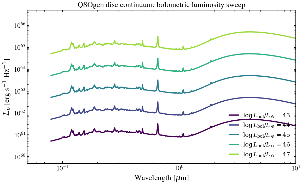
QSOgen Disc Continuum: Bolometric Luminosity

Sweep log L_bol / L_sun from 43 to 47 on the QSOgen disc continuum. The continuum normalisation tracks luminosity directly; the disc temperature shifts more subtly with the implied accretion rate.

import jax.numpy as jnp
import matplotlib.pyplot as plt
import numpy as np

from tengri.analysis.plotting import setup_style
from tengri.components.agn import qsogen

setup_style()

# Wavelength grid: UV to NIR (800 - 100,000 Angstrom)
wavelength = jnp.logspace(np.log10(800), np.log10(1e5), 512)
wave_um = np.array(wavelength) / 1e4

# Bolometric luminosity values to sweep
log_lbol_values = [43, 44, 45, 46, 47]

# Create figure with single panel
fig, ax = plt.subplots(figsize=(8, 5))

# Generate colors from colormap
colors = plt.cm.viridis(np.linspace(0.0, 0.85, len(log_lbol_values)))

# Sweep — plot absolute L_nu so the four-decade L_bol shift is visible.
# Each curve at log L_bol = X sits 10x above log L_bol = X-1.
for log_lbol, color in zip(log_lbol_values, colors):
    sed = np.array(qsogen(wavelength, agn_log_lbol=log_lbol))
    sed_safe = np.where(sed > 0, sed, np.nan)
    label = rf"$\log L_{{\mathrm{{bol}}}}/L_\odot = {log_lbol}$"
    ax.loglog(wave_um, sed_safe, lw=2.2, color=color, label=label)

ax.set_xlabel(r"Wavelength [$\mu$m]")
ax.set_ylabel(r"$L_\nu$ [erg s$^{-1}$ Hz$^{-1}$]")
ax.set_title("QSOgen disc continuum: bolometric luminosity sweep", fontsize=14)
ax.legend(fontsize=11, frameon=False, loc="lower right")
# Broad zoomed-out view of the QSOgen rest-frame SED, covering Lyα forest
# (~0.05 µm) through NIR turnover (~5 µm). 7 decades of L_nu give breathing
# room for all 5 luminosity curves.
ax.set_xlim(0.05, 10.0)
ax.set_ylim(5e59, 5e66)
ax.grid(False)

fig.tight_layout()
plt.savefig("plot_agn_log_lbol_sweep.png", dpi=150, bbox_inches="tight")
plt.show()