Note
Go to the end to download the full example code.
Compton hump in obscured AGN: pexrav reflection across log N_H
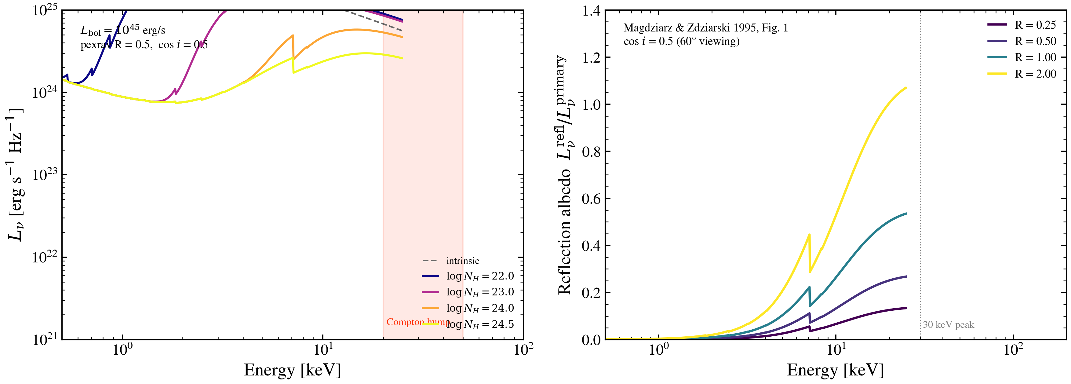
In Compton-thick AGN (log N_H ≳ 24 cm⁻²), the line-of-sight obscurer extinguishes the primary AGN corona below ~ 10 keV. What’s left is the reflected component — the fraction of corona photons that hit the cold accretion disc, Compton-scatter off bound electrons, and emerge along the line of sight without being photoelectrically absorbed. The resulting spectrum peaks around 30 keV (the famous Compton hump) and is the smoking-gun signature that NuSTAR / Swift-BAT surveys use to confirm buried supermassive black holes (Ricci+2017, Matsumoto+26).
This example uses pexrav_reflection (Magdziarz & Zdziarski 1995)
through the public xray_agn_corona API. The reflection albedo
arises from the σ_T / (σ_T + σ_phabs(E)) branching ratio: at low E
the disc photoelectrically absorbs everything, at high E Compton
wins and the photons are scattered back to the observer.
Left panel: full Ricci+2017 / Matsumoto+26 Eq. B6 model:
swept through log N_H = 22 → 24.5. The Compton hump emerges as the primary continuum dims into Compton-thick obscuration.
Right panel: reflection albedo (L_refl / L_intr) for different covering fractions R, reproducing the MZ95 Fig. 1 shape.
References
Magdziarz & Zdziarski 1995, MNRAS 273, 837 (pexrav, XSPEC).
Ricci et al. 2017, Nature 549, 488 (R=0.5 obscured-AGN spectral model).
Matsumoto et al. 2026, Appendix B (Eq. B6 fits at z > 3).
import warnings

import jax.numpy as jnp
import matplotlib as mpl
import matplotlib.pyplot as plt
import numpy as np

from tengri.plot import setup_style
from tengri.xray import pexrav_reflection, xray_agn_corona

setup_style()
warnings.filterwarnings("ignore", message=".*BakedInBackend.*")

# ------------------------------------------------------------------- grid
wave = jnp.logspace(np.log10(0.5), np.log10(124.0), 1024)
E_keV = 12.398 / np.asarray(wave)

L_BOL = 1e45  # erg/s — luminous local AGN
L_2500 = L_BOL / (5.15 * 1.199e15)  # Hopkins+2007 BC_2500 → erg/s/Hz

# ------------------------------------------------------------------- figure
fig, axes = plt.subplots(1, 2, figsize=(12, 4.5))

# (a) Full obscured AGN spectrum across log N_H, with reflection on
ax = axes[0]
nh_grid = np.array([22.0, 23.0, 24.0, 24.5])
cmap = plt.get_cmap("plasma")
norm = mpl.colors.Normalize(vmin=22.0, vmax=24.5)

# Intrinsic (unabsorbed, no reflection) baseline
L_intr = np.asarray(
    xray_agn_corona(
        wave,
        l_2500_30deg_erg_hz=L_2500,
        log_nh=15.0,
        pexrav_R=0.0,
        apply_anisotropy=False,
    )
)
ax.loglog(E_keV, L_intr, color="0.4", ls="--", lw=1.2, label="intrinsic")

for log_nh in nh_grid:
    L = np.asarray(
        xray_agn_corona(
            wave,
            l_2500_30deg_erg_hz=L_2500,
            log_nh=log_nh,
            pexrav_R=0.5,
            apply_anisotropy=False,
        )
    )
    ax.loglog(
        E_keV,
        L,
        color=cmap(norm(log_nh)),
        lw=1.6,
        label=rf"$\log N_H = {log_nh:.1f}$",
    )

ax.set_xlim(0.5, 100)
ax.set_ylim(1e21, 1e25)
ax.set_xlabel("Energy [keV]")
ax.set_ylabel(r"$L_\nu$ [erg s$^{-1}$ Hz$^{-1}$]")
ax.axvspan(20.0, 50.0, alpha=0.10, color="C3")
ax.text(30.0, 1.5e21, "Compton hump", color="C3", fontsize=8, ha="center")
ax.text(
    0.04,
    0.96,
    f"$L_{{\\rm bol}} = 10^{{{np.log10(L_BOL):.0f}}}$ erg/s\npexrav R = 0.5,  cos $i$ = 0.5",
    transform=ax.transAxes,
    va="top",
    fontsize=9,
)
ax.legend(fontsize=8, frameon=False, loc="lower right")

# (b) Reflection albedo for different R
ax = axes[1]
R_grid = np.array([0.25, 0.5, 1.0, 2.0])
cmap2 = plt.get_cmap("viridis")
norm2 = mpl.colors.Normalize(vmin=R_grid.min(), vmax=R_grid.max())
unit_primary = jnp.ones_like(wave)

for R in R_grid:
    A = np.asarray(pexrav_reflection(wave, unit_primary, R=float(R), cos_inc=0.5))
    ax.semilogx(E_keV, A, color=cmap2(norm2(R)), lw=1.8, label=f"R = {R:.2f}")

ax.axvline(30.0, color="0.5", ls=":", lw=0.8)
ax.text(31.0, 0.05, "30 keV peak", color="0.5", fontsize=8)
ax.set_xlim(0.5, 200)
ax.set_ylim(0.0, 1.4)
ax.set_xlabel("Energy [keV]")
ax.set_ylabel(r"Reflection albedo  $L_\nu^{\rm refl} / L_\nu^{\rm primary}$")
ax.text(
    0.04,
    0.96,
    "Magdziarz & Zdziarski 1995, Fig. 1\ncos $i$ = 0.5 (60° viewing)",
    transform=ax.transAxes,
    va="top",
    fontsize=9,
)
ax.legend(fontsize=9, frameon=False, loc="upper right")

fig.tight_layout()
plt.savefig("plot_xray_pexrav_compton_hump.png", dpi=150, bbox_inches="tight")