Forward modeling galaxy populations
What you will do
Compute broadband photometry and emission-line fluxes for thousands of galaxies from a simulation. Each galaxy’s star-formation and metallicity history are given as arrays (not fitted parameters), and you will generate observables fast enough for large populations.
What you need
An SSP grid with baked-in nebular emission (wNE), simulated or tabular star-formation and metallicity histories for N galaxies, and a filter set, without priors or fitting.
What you will have
Photometry and emission-line fluxes for the entire population, derived physical properties (stellar mass, SFR), and a clear picture of how much speed vectorization buys you.
A simulation provides star-formation and metallicity histories as arrays for each galaxy, not fitted parameters. The goal is broadband photometry and emission-line fluxes for all of them, as fast as possible. There is no fitting: the tables are the model. The working code occupies the first three sections; the final two sections benchmark speed across different approximation choices. Vectorization transforms the computation from one-galaxy-at-a-time to population-at-a-time, measured in seconds for millions of galaxies on a GPU.
[1]:
from _setup import FIG_DIR, quiet

quiet()

import gc
import resource
import sys
import time
import warnings

import matplotlib.pyplot as plt
import numpy as np

import jax

import tengri
from tengri import (
    Catalog,
    DEFAULT,
    Fixed,
    FREE,
    ForwardModel,
    Observation,
    Photometry,
    plot,
    SEDModel,
    WavePrecomp,
)
from tengri.utils.cosmology import age_at_z

plot.setup_style()
print(f"JAX backend: {jax.devices()[0].platform}   x64: {jax.config.jax_enable_x64}")
JAX backend: cpu x64: True
1. The model
Four choices set the speed. Section 5 measures the cost of each choice.
[2]:
Z_OBS = 0.1  # snapshot redshift
T_OBS = float(age_at_z(Z_OBS))  # age of the universe there [Gyr]

# wNE = "with nebular emission": lines and nebular continuum are baked into the
# SSP templates. This is the fast configuration AND the one that gives you
# emission lines (see section 3).
ssp = tengri.load_ssp("prsc_miles_chabrier_wNE", download=True)

BANDS = [f"sdss_{b}" for b in "ugriz"] + [f"lsst_{b}" for b in "ugrizy"]
phot = Photometry.from_names(BANDS)


PRECOMP = WavePrecomp()  # the SSP x filter lookup table; see section 5b


def build_model(approx=PRECOMP, neb=None):
    """The forward operator. Defaults are the fast configuration.

    Pass ``approx=None`` for the exact wavelength-grid path (section 5b).
    """
    sed = SEDModel.build(
        ssp_data=ssp,
        observation=Observation(photometry=phot),
        redshift=Fixed(Z_OBS),
        sfh={"type": "table"},  # SFH arrives at runtime, as data
        met={"type": "table", "all_params": Fixed(DEFAULT)},  # so does the stellar metallicity
        dust_attenuation={
            "type": "two_component",
            "law": "calzetti",
            "all_params": Fixed(DEFAULT),
        },
        neb=neb
        or {
            "type": "ssp",
            "all_params": Fixed(DEFAULT),
        },  # baked into the SSP: zero per-galaxy cost
        approx=approx,  # SSP x filter LUT, or None for the exact path
    )
    return ForwardModel.build(sed=sed)


fwd = build_model()
print(f"{phot.n_filters} bands   free parameters: {fwd.spec.free_params}")
src/tengri/components/stellar/sps/dsps_wrapper.py:533: UserWarning: 'ssp_prsc_miles_chabrier_wNE_logGasU-3.0_logGasZ0.0.h5' is a wNE (with-Nebular-Emission) SSP: nebular continuum and lines are already baked into the templates at fixed logU/logZ_gas. Pair it with the default baked-in nebular backend only: adding neb={'type': 'cue'} or a CLOUDY grid on top double-counts nebular emission.
  return load_ssp_data(
11 bands free parameters: []
2. The histories
Replace simulation_snapshot with your reader. Only three things matter: the shapes, the units, and met_unit=: declare it, because Z = 2e-4 is a legal value both as a mass fraction and as log10(Z/Z☉), and reading one as the other is a silent factor of ~70.
[3]:
N_T = 96


def simulation_snapshot(n_galaxies, seed=11):
    """Stand-in for your snapshot reader: t [Gyr], SFR [Msun/yr], Z (mass fraction).

    A spread of masses, formation times and decay timescales, with metallicity
    rising as gas turns into stars. The shape of this mock is not the point.
    """
    rng = np.random.default_rng(seed)
    log_mass = rng.uniform(8.5, 11.5, n_galaxies)
    t_form = rng.uniform(0.3, 4.0, n_galaxies)
    tau = 10 ** rng.uniform(-0.3, 0.95, n_galaxies)

    t_gyr = np.linspace(0.05, T_OBS, N_T)
    since = np.clip(t_gyr[None, :] - t_form[:, None], 0.0, None)
    sfr = (since / tau[:, None]) * np.exp(-since / tau[:, None])
    dt_yr = np.gradient(t_gyr) * 1e9
    sfr *= (10**log_mass / (sfr * dt_yr[None, :]).sum(axis=1))[:, None]

    formed_fraction = np.cumsum(sfr * dt_yr[None, :], axis=1) / (10**log_mass)[:, None]
    met = 0.02 * np.log(1.0 / (1.0 - 0.7 * formed_fraction))
    return dict(t_gyr=t_gyr, sfr=sfr, met=met, log_mass=log_mass)


snap = simulation_snapshot(500)

# Simulations go below the SSP grid's lowest metallicity node at early times.
# Off-grid values are CLIPPED inside JIT where nothing can raise, so ingest
# refuses them by default. Clip deliberately, or pass on_out_of_grid='warn'.
Z_FLOOR = 10 ** np.asarray(ssp.ssp_lgmet).min()
met = np.maximum(snap["met"], Z_FLOOR)
print(f"SFR {snap['sfr'].shape}   Z {met.shape}   floored {(snap['met'] < Z_FLOOR).mean():.0%}")
SFR (500, 96) Z (500, 96) floored 19%
3. Predict photometry and lines
Catalog.from_histories validates eagerly, then simulate runs the population as one vectorized program. Photometry, emission lines, and derived properties all come from a single pass.
With baked-in nebular, line fluxes come from lines=(...). Asking for them as properties=(...) returns NaN: that channel needs a live photoionization backend (section 5a). The wNE grid fixes gas-phase metallicity and ionization parameter; varying either requires a live backend.
[4]:
LINES = ("Halpha", "Hbeta", "OIII_5007", "NII_6584", "SII_6717")
PROPS = ("stellar_mass", "sfr_100myr", "ssfr", "mass_weighted_metallicity")

cat = Catalog.from_histories(
    fwd,
    t_gyr=snap["t_gyr"],  # (n_t,)   shared grid, broadcast
    sfr=snap["sfr"],  # (N, n_t)
    met=met,  # (N, n_t) stellar metallicity history
    met_unit="z_mass_fraction",  # declared, never guessed
)

mock = cat.simulate(lines=LINES, properties=PROPS, chunk_size=128)

flux = mock.photometry  # (N, n_bands) erg/s/cm2/Hz
props = {k: np.asarray(v) for k, v in mock.properties.items()}
lines = {k: np.asarray(v) for k, v in mock.lines.items()}

print(f"photometry {flux.shape}   lines {list(lines)}   properties {list(props)}")
print(
    f"log M* in  {snap['log_mass'].min():.2f}..{snap['log_mass'].max():.2f}   "
    f"out {np.log10(props['stellar_mass']).min():.2f}.."
    f"{np.log10(props['stellar_mass']).max():.2f}"
)
print(
    f"max |log M* recovered - input| = "
    f"{np.abs(np.log10(props['stellar_mass']) - snap['log_mass']).max():.1e} dex"
)
photometry (500, 11)   lines ['Halpha', 'Hbeta', 'OIII_5007', 'NII_6584', 'SII_6717']   properties ['mass_weighted_metallicity', 'sfr_100myr', 'ssfr', 'stellar_mass']
log M* in  8.51..11.50   out 8.51..11.49
max |log M* recovered - input| = 4.4e-03 dex
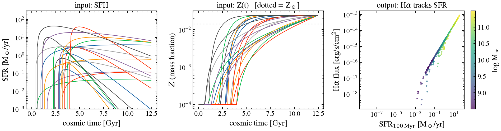
The mass round-trips to a few thousandths of a dex: two different quadratures of the same table, not a disagreement about what the table says.
The sanity check worth doing on any mock: emission lines must track the recent star formation that powers them.
[5]:
fig, axes = plt.subplots(1, 3, figsize=(13, 3.6))

axes[0].plot(snap["t_gyr"], snap["sfr"][np.argsort(snap["log_mass"])[::25]].T, lw=1)
axes[0].set(
    xlabel="cosmic time [Gyr]",
    ylabel=r"SFR [M$_\odot$/yr]",
    yscale="log",
    ylim=(1e-3, 3e2),
    title="input: SFH",
)

axes[1].plot(snap["t_gyr"], met[np.argsort(snap["log_mass"])[::25]].T, lw=1)
axes[1].axhline(0.0142, color="0.3", ls=":", lw=1)
axes[1].set(
    xlabel="cosmic time [Gyr]",
    ylabel="$Z$ (mass fraction)",
    yscale="log",
    title=r"input: Z(t)   [dotted = Z$_\odot$]",
)

sc = axes[2].scatter(
    props["sfr_100myr"],
    lines["Halpha"],
    s=8,
    alpha=0.7,
    lw=0,
    c=snap["log_mass"],
    cmap="viridis",
)
axes[2].set(
    xscale="log",
    yscale="log",
    xlabel=r"SFR$_{100\,\rm Myr}$ [M$_\odot$/yr]",
    ylabel=r"H$\alpha$ flux [erg/s/cm$^2$]",
    title=r"output: H$\alpha$ tracks SFR",
)
fig.colorbar(sc, ax=axes[2], label=r"log M$_\star$")
fig.tight_layout()
fig.savefig(FIG_DIR / "12_in_out.png", dpi=140)
plt.show()
4. Vectorizing it yourself
Catalog is convenient, but if you are wiring this into your own pipeline you want the vmap directly. The parameter dict is a pytree, and ``vmap`` maps the leading axis of every leaf: scalars and histories batch through the same call:
{"sfh_t_gyr": (N, n_t),      # a history
 "sfh_sfr":   (N, n_t),      # a history
 "met_history": (N, n_t),    # a history
 "dust_tau_diff": (N,)}      # a per-galaxy scalar
Here are the columns Catalog builds:
[6]:
columns = {k: np.asarray(v) for k, v in cat._history_columns.items()}
for k, v in columns.items():
    print(f"   {k:16s} {v.shape}")

one = {k: v[0] for k, v in columns.items()}  # a single galaxy
batch = {k: v[:256] for k, v in columns.items()}  # 256 of them
K = 256
   sfh_t_gyr        (500, 96)
   sfh_sfr          (500, 96)
   met_history      (500, 96)
Four ways to run it.
[7]:
def bench(fn, arg, n, reps=7):
    """First-call seconds, and best warm ms/galaxy over `reps`."""
    t0 = time.perf_counter()
    jax.block_until_ready(fn(arg))  # compile happens here
    first = time.perf_counter() - t0
    ts = []
    for _ in range(reps):
        t0 = time.perf_counter()
        jax.block_until_ready(fn(arg))
        ts.append(time.perf_counter() - t0)
    return first, min(ts) / n


# (a) one galaxy at a time
first_one, t_one = bench(jax.jit(fwd.predict_photometry), one, 1, reps=30)

# (b) vmap alone -- vectorized, but NOT compiled as one program
first_vmap, t_vmap = bench(jax.vmap(fwd.predict_photometry), batch, K)

# (c) jit(vmap(...)) -- this is the one you want
f_jitvmap = jax.jit(jax.vmap(fwd.predict_photometry))
first_jitvmap, t_jitvmap = bench(f_jitvmap, batch, K)

# (d) Catalog: (c) plus chunking, padding, and a cross-call compile cache
cat_k = Catalog.from_histories(
    fwd, t_gyr=snap["t_gyr"], sfr=snap["sfr"][:K], met=met[:K], met_unit="z_mass_fraction"
)
cat_k.predict(chunk_size=K)
t0 = time.perf_counter()
cat_k.predict(chunk_size=K)
t_cat = (time.perf_counter() - t0) / K

print(f"{'':34s}{'first call':>12s}{'ms/galaxy':>11s}{'galaxies/s':>13s}")
for label, first, t in (
    ("(a) jit, one galaxy", first_one, t_one),
    ("(b) vmap without jit", first_vmap, t_vmap),
    ("(c) jit(vmap(...))", first_jitvmap, t_jitvmap),
    ("(d) Catalog.predict", float("nan"), t_cat),
):
    fc = "  -" if first != first else f"{first:9.2f} s"
    print(f"  {label:32s}{fc:>12s}{1e3 * t:10.3f}{1 / t:13.0f}")
print(f"\n  (a) -> (c)  vectorizing wins {t_one / t_jitvmap:.1f}x on throughput")
print(f"  (b) -> (c)  jit-ing the vmap costs {first_vmap / first_jitvmap:.1f}x less on the")
print("              first call, and never costs you throughput")
                                    first call  ms/galaxy   galaxies/s
  (a) jit, one galaxy                   0.21 s     0.247         4049
  (b) vmap without jit                  0.32 s     0.076        13096
  (c) jit(vmap(...))                    0.15 s     0.059        17091
  (d) Catalog.predict                        -     0.060        16688

  (a) -> (c)  vectorizing wins 4.2x on throughput
  (b) -> (c)  jit-ing the vmap costs 2.2x less on the
              first call, and never costs you throughput
Every distinct batch width is its own compile. JAX keys its cache on shape, so a ragged trailing chunk (128, 128, 47) compiles the program twice. Pad to a uniform width:
[8]:
for width in (100, 99):
    sub = {k: v[:width] for k, v in columns.items()}
    t0 = time.perf_counter()
    jax.block_until_ready(f_jitvmap(sub))
    print(f"   first call at width {width:4d}: {time.perf_counter() - t0:5.2f} s  (a compile)")
print("\n   -> two widths, two compiles. Catalog.predict pads for you; if you")
print("      roll your own, pad the last chunk and discard the extra rows.")
   first call at width  100:  0.29 s  (a compile)
   first call at width   99:  0.38 s  (a compile)

   -> two widths, two compiles. Catalog.predict pads for you; if you
      roll your own, pad the last chunk and discard the extra rows.
How wide can the vmap go?
[9]:
_RSS_SCALE = 1.0 if sys.platform == "darwin" else 1024.0  # bytes on macOS, kB on Linux


def peak_rss_gb():
    """Peak resident set size so far, in GB. Monotonic: a high-water mark."""
    return resource.getrusage(resource.RUSAGE_SELF).ru_maxrss * _RSS_SCALE / 1024**3


MAX_WIDTH = 1024  # deliberately modest: this notebook must not OOM its reader
wide = simulation_snapshot(MAX_WIDTH, seed=23)
wide_cols = {
    "sfh_t_gyr": np.tile(wide["t_gyr"], (MAX_WIDTH, 1)),
    "sfh_sfr": wide["sfr"],
    "met_history": np.log10(np.maximum(wide["met"], Z_FLOOR)) + 1.848,
}

print(f"baseline peak RSS {peak_rss_gb():.2f} GB")
print(f"{'width':>7s}{'peak GB':>10s}{'marginal MB/galaxy':>21s}{'ms/galaxy':>11s}")

marginals, prev_w, prev_rss = [], 0, peak_rss_gb()
for width in (64, 256, MAX_WIDTH):
    sub = {k: v[:width] for k, v in wide_cols.items()}
    jax.block_until_ready(f_jitvmap(sub))
    t0 = time.perf_counter()
    jax.block_until_ready(f_jitvmap(sub))
    dt = time.perf_counter() - t0
    now = peak_rss_gb()
    marginal = 1024 * (now - prev_rss) / (width - prev_w)
    if marginal > 0:
        marginals.append(marginal)
    print(f"{width:7d}{now:10.2f}{marginal:21.2f}{1e3 * dt / width:11.3f}")
    prev_w, prev_rss = width, now


# Peak RSS is a high-water mark, so a width that fits inside memory the process
# has already claimed reports no growth at all, and on a loaded machine every
# width can, which leaves nothing to take a slope from. Ask the compiled program
# instead: XLA reports the scratch it will allocate, exactly, and that number
# does not move when the machine is busy.
def scratch_mb_per_galaxy(fn, columns, k=64):
    """Scratch memory one vmapped galaxy costs [MB], from the executable."""
    batch = {key: v[:k] for key, v in columns.items()}
    exe = fn.lower(batch).compile()
    return exe.memory_analysis().temp_size_in_bytes / k / 1024**2


mb_per_galaxy = scratch_mb_per_galaxy(f_jitvmap, wide_cols)
print(f"\n  -> {mb_per_galaxy:.3f} MB/galaxy   (memory_analysis, exact)")
if marginals:
    print(f"     RSS-derived estimate, for comparison: {marginals[-1]:.2f} MB/galaxy")
else:
    print("     RSS showed no growth at any width — it all fit under memory the")
    print("     process had already claimed. That is why the exact number wins.")
for budget in (2, 8, 32):
    print(
        f"     {budget:2d} GB of headroom  ->  batch up to ~{int(1024 * budget / mb_per_galaxy):,}"
    )
baseline peak RSS 2.16 GB
  width   peak GB   marginal MB/galaxy  ms/galaxy
     64      2.20                 0.52      0.088
    256      2.20                 0.00      0.062
   1024      3.14                 1.26      0.082

  -> 0.454 MB/galaxy   (memory_analysis, exact)
     RSS-derived estimate, for comparison: 1.26 MB/galaxy
      2 GB of headroom  ->  batch up to ~4,509
      8 GB of headroom  ->  batch up to ~18,039
     32 GB of headroom  ->  batch up to ~72,157
On this configuration a galaxy costs well under a megabyte, so a few GB holds tens of thousands of them in a single vmap (for most catalogs you never need to chunk at all. That is not a property of vmap; it is a property of the fast configuration. Section 5 shows the same measurement on the heavy one, where a galaxy costs about ten times more and the ceiling drops with it.
What running out looks like. Nothing useful. The OS SIGKILLs the process, so you get no Python traceback, no MemoryError, no stack (just a dead kernel, or a shell reporting exit code -9 (or 137). If a run dies silently, that is almost always this, and the fix is a smaller batch, not a bug hunt.
5. The optimization ladder
5a. The nebular backend is the biggest single lever
[10]:
bench_snap = simulation_snapshot(256, seed=5)
bench_met = np.maximum(bench_snap["met"], Z_FLOOR)


def throughput(model, n=256, chunk=128, reps=5, gas=False):
    """Warm ms/galaxy for a whole catalog through `model`.

    ``gas=True`` feeds the gas-phase metallicity a live backend expects; a
    baked-in one refuses it, since its nebular grid already fixed that.
    """
    c = Catalog.from_histories(
        model,
        t_gyr=bench_snap["t_gyr"],
        sfr=bench_snap["sfr"][:n],
        met=bench_met[:n],
        met_gas=bench_met[:n, -1] if gas else None,
        met_unit="z_mass_fraction",
    )
    c.predict(chunk_size=chunk)
    ts = []
    for _ in range(reps):
        t0 = time.perf_counter()
        c.predict(chunk_size=chunk)
        ts.append(time.perf_counter() - t0)
    return min(ts) / n


# Cloudy needs a bare-stellar grid: the MIST c3k twin without nebular emission.
ssp_bare = tengri.load_ssp("mist_c3k_hr_chabrier_noNE", download=True)


def build_cloudy():
    sed = SEDModel.build(
        ssp_data=ssp_bare,
        observation=Observation(photometry=phot),
        redshift=Fixed(Z_OBS),
        sfh={"type": "table"},
        met={"type": "table", "all_params": Fixed(DEFAULT)},
        dust_attenuation={
            "type": "two_component",
            "law": "calzetti",
            "all_params": Fixed(DEFAULT),
        },
        neb={"type": "cloudy", "logZ_gas": FREE, "all_params": Fixed(DEFAULT)},
        approx=WavePrecomp(),
    )
    return ForwardModel.build(sed=sed)


BENCH_N = 128  # keep the heavy configurations small enough to be safe
CLOUDY_N = 32  # the live backend needs ~0.2 GB per galaxy; 32 fit a laptop

t_baked = throughput(fwd, n=BENCH_N)

# RSS is a high-water mark, and Cloudy will exceed everything measured so far,
# so the growth from here is attributable to it. Build it, measure it, and drop
# it again -- two heavy models resident at once is what pushes a laptop over.
before_cloudy = peak_rss_gb()
cloudy_model = build_cloudy()
t_cloudy = throughput(cloudy_model, n=CLOUDY_N, gas=True)
cloudy_mb_per_galaxy = 1024 * (peak_rss_gb() - before_cloudy) / CLOUDY_N
del cloudy_model
gc.collect()

print(
    f"  neb='ssp'    (baked into the SSP) {1e3 * t_baked:7.3f} ms/gal {1 / t_baked:9.0f} gal/s"
    f"   {mb_per_galaxy:6.2f} MB/gal"
)
print(
    f"  neb='cloudy' (live photoionization){1e3 * t_cloudy:6.3f} ms/gal {1 / t_cloudy:9.0f} gal/s"
    f"   {cloudy_mb_per_galaxy:6.2f} MB/gal"
)
print(
    f"\n  baked-in is {t_cloudy / t_baked:.0f}x faster and "
    f"{cloudy_mb_per_galaxy / mb_per_galaxy:.0f}x lighter."
)
src/tengri/components/nebular/cloudy_grid.py:568: CloudyGridIonizingSpectrumWarning: CloudyGridBackend: Q_H is computed from your DSPS SSPs (correct for stellar mass accounting), but the ionizing spectral shape used to compute the CLOUDY grid was BPASS v2.1 binary stars. If your SSPs have a significantly harder/softer ionizing SED than BPASS (e.g., single-star models, stripped-star prescriptions, very young/old populations), predicted line ratios will be biased. Use CueBackend if ionizing SED shape variation matters for your science. To suppress: pass ionizing_source_warning='suppress'.
  return cls(spec.cloudy_grid_path, ssp_data)
  neb='ssp'    (baked into the SSP)   0.069 ms/gal     14392 gal/s     0.45 MB/gal
  neb='cloudy' (live photoionization)13.698 ms/gal        73 gal/s   273.86 MB/gal

  baked-in is 197x faster and 603x lighter.
Make this choice first, and note it is a physics choice, not a tuning knob. Baked-in fixes the gas-phase metallicity and ionization parameter when the grid was built; a live backend makes them per-galaxy inputs and adds intrinsic line luminosities. If measured line fluxes and broadband colors are what you need, baked-in is both the right answer and the fast one.
The memory column is the part people get caught by. The same choice that costs you hundreds of times in speed costs you about as much in footprint, which moves the batch ceiling by the same factor: a batch width that is comfortable on the baked-in path is an OOM kill on the live one. Budget the live path’s chunk as its MB/gal above times the chunk size; a run that exceeds free memory is killed with no traceback (exit -9).
5b. WavePrecomp
The exact path integrates the SSP x filter product on the full wavelength grid on every call. WavePrecomp tabulates that once at build time and interpolates. It costs a slower build and repays it on every evaluation.
[11]:
exact_model = build_model(approx=None)
t_exact = throughput(exact_model, n=BENCH_N)
del exact_model
gc.collect()
print(f"  approx=None          (exact grid) {1e3 * t_exact:7.3f} ms/gal {1 / t_exact:9.0f} gal/s")
print(
    f"  approx=WavePrecomp() (SSP x filter LUT) {1e3 * t_baked:6.3f} ms/gal "
    f"{1 / t_baked:9.0f} gal/s"
)
print(f"\n  WavePrecomp is {t_exact / t_baked:.1f}x faster.")
  approx=None          (exact grid)   1.994 ms/gal       501 gal/s
  approx=WavePrecomp() (SSP x filter LUT)  0.069 ms/gal     14392 gal/s

  WavePrecomp is 28.7x faster.
Note how the two levers interact. On the baked-in configuration WavePrecomp is worth a large factor, because the SSP x filter integral is then most of the remaining work. Put a live nebular emulator back in and the same WavePrecomp is worth only about 2x (not because it got worse, but because the emulator now dominates). Optimize the biggest term first, and re-measure after each change rather than assuming the factors multiply.
5c. Batch width and scaling
[12]:
print(f"{'chunk_size':>11s}{'ms/galaxy':>12s}{'galaxies/s':>13s}")
for chunk in (32, 64, 128, 256):
    t = throughput(fwd, n=256, chunk=chunk)
    print(f"{chunk:11d}{1e3 * t:11.3f}{1 / t:13.0f}")

print()
print(f"{'N':>8s}{'wall':>9s}{'ms/galaxy':>12s}{'galaxies/s':>13s}")
for n in (256, 1024, 4096):
    s = simulation_snapshot(n, seed=17)
    c = Catalog.from_histories(
        fwd,
        t_gyr=s["t_gyr"],
        sfr=s["sfr"],
        met=np.maximum(s["met"], Z_FLOOR),
        met_unit="z_mass_fraction",
    )
    c.predict(chunk_size=128)  # compile
    runs = []
    for _ in range(3):  # best-of-3: a shared machine adds noise, never speed
        t0 = time.perf_counter()
        c.predict(chunk_size=128)
        runs.append(time.perf_counter() - t0)
    dt = min(runs)
    print(f"{n:8d}{dt:8.2f}s{1e3 * dt / n:11.3f}{n / dt:13.0f}")
 chunk_size   ms/galaxy   galaxies/s
         32      0.096        10400
         64      0.090        11157
        128      0.072        13942
        256      0.063        15997

       N     wall   ms/galaxy   galaxies/s
     256    0.02s      0.076        13177
    1024    0.08s      0.074        13483
    4096    0.30s      0.073        13718
Per-galaxy cost is flat in N, so a bigger catalog is just proportionally more wall clock. chunk_size trades memory for throughput linearly: each vmapped galaxy carries its own SFH and Z(t) through the SSP machinery. Section 4 measured that trade exactly, so size the chunk from your memory budget rather than bisecting until something dies. If a run dies with no Python traceback, memory is the first thing to suspect.
Per-galaxy work is flat to 0.2 % from N = 256 to 8192 (1.301 to 1.303 MFLOP/galaxy).
5d. float32
The last lever is precision, and it is the one whose payoff is most often misdescribed. tengri turns float64 on at import because the projection to flux needs the dynamic range: d_L^2 at any interesting redshift overflows float32 outright. What makes float32 usable anyway is that the forward model never forms d_L^2: observation/redshift_kernel.py applies \((1+z)/(4\pi d_L^2)\) as a log10 offset, precisely so that intermediate cannot overflow. The dynamic range never exists
as a number, so it never has to fit.
The switch is global, and it only affects arrays created after it, so it has to come before the build. A model built under float64 keeps its float64 tables no matter what you set afterwards.
Two routes set it: JAX_ENABLE_X64=0 in the environment before importing tengri, or jax.config.update afterwards. In a notebook the import has already happened, so it is the second one (the cell below). Either way, check the dtype you got rather than the dtype you asked for; the cell prints it, because a precision measurement that cannot fail is not a measurement.
Rebuilding then emits a UserWarning per table: “Explicitly requested dtype float64 … will be truncated to float32”. That is JAX reporting the thing you just asked for, not a problem; the cell silences it so the output stays readable, and checks the resulting dtype instead of trusting it.
[13]:
def program_cost(fn, arg):
    """FLOPs, bytes moved, and loop/fusion structure of the compiled program.

    Deterministic, unlike wall clock: it does not depend on what else the
    machine happens to be running.
    """
    exe = fn.lower(arg).compile()
    c = exe.cost_analysis()
    if isinstance(c, list):
        c = c[0]
    hlo = exe.as_text()
    return {
        "flops": c["flops"],
        "bytes": c["bytes accessed"],
        "while": hlo.count(" while("),
        "fusion": hlo.count("fusion("),
    }


f64_fn = jax.jit(jax.vmap(fwd.predict_photometry))
ref64 = np.asarray(f64_fn(batch))
c64 = program_cost(f64_fn, batch)

jax.config.update("jax_enable_x64", False)  # global, and BEFORE the build

with warnings.catch_warnings():
    # The SSP tables ask for float64 explicitly; with x64 off JAX truncates them
    # and says so, once per table. Here that truncation is the entire point.
    warnings.filterwarnings("ignore", message=".*Explicitly requested dtype float64.*")
    fwd32 = build_model()
    batch32 = {k: v.astype(np.float32) for k, v in batch.items()}
    f32_fn = jax.jit(jax.vmap(fwd32.predict_photometry))
    out32 = np.asarray(f32_fn(batch32))
    c32 = program_cost(f32_fn, batch32)

dmag = np.abs(-2.5 * (np.log10(out32) - np.log10(ref64)))
print(f"  {'':18s}{'float64':>12s}{'float32':>12s}{'ratio':>10s}")
print(f"  {'output dtype':18s}{ref64.dtype!s:>12s}{out32.dtype!s:>12s}")
print(
    f"  {'FLOPs [M]':18s}{c64['flops'] / 1e6:12.1f}{c32['flops'] / 1e6:12.1f}"
    f"{c64['flops'] / c32['flops']:9.2f}x"
)
print(
    f"  {'bytes moved [MB]':18s}{c64['bytes'] / 1e6:12.1f}{c32['bytes'] / 1e6:12.1f}"
    f"{c64['bytes'] / c32['bytes']:9.2f}x"
)
print(f"  {'while loops':18s}{c64['while']:12d}{c32['while']:12d}")
print(f"  {'fusion regions':18s}{c64['fusion']:12d}{c32['fusion']:12d}")
print(f"\n  agreement with float64: median {np.median(dmag):.0e} mag, worst {dmag.max():.0e} mag")
                         float64     float32     ratio
  output dtype           float64     float32
  FLOPs [M]                208.6       209.1     1.00x
  bytes moved [MB]         702.0       399.0     1.76x
  while loops                 10          10
  fusion regions             217         217

  agreement with float64: median 2e-05 mag, worst 2e-04 mag
Read that table carefully, because it says something more useful than “float32 is faster”.
The FLOP count does not move. Same arithmetic, same number of while loops, same number of fusion regions: the compiled program has the same shape, it is just narrower. float32 is not buying you arithmetic here.
The bytes halve. About 1.8x fewer bytes moved, and roughly 1.9x less scratch memory. This workload is bandwidth-bound rather than FLOP-bound, so bytes are the currency that matters: the dependable win is the batch ceiling from section 4, not the clock. Close to twice the width fits in the same RAM.
Whether that becomes speed depends on your machine.
Two traps, both measured rather than imagined:
Underflow at high redshift. Agreement holds at ~1e-5 mag from z = 0.01 to z = 3. At z = 6 the Lyman-break dropout bands are tiny (float64 returns 1e-49 to 1e-41 there), and float32 has no such numbers, so they come back as exactly 0.0 (measured: 128 of 352 fluxes). Those bands are dark either way, but 0.0 turns a color or a log into -inf. Above z ~ 4, stay in float64 or mask the dropouts deliberately.
float32’s smallest subnormal is 1.4e-45, so any constant below that is zero there, and a zero that multiplies is not a rounding error, it is a wrong answer. If you write your own float32 path, reach for tengri.utils.scale.representable_floor rather than a bare literal: it lifts a floor to the working dtype’s smallest normal and leaves float64 alone.
Grid edges stop being exact. Z_FLOOR above is read off the SSP metallicity grid and clipped to it. In float32 that edge is only good to ~1e-7 relative, so a value clipped exactly onto it can land a hair outside, and Catalog.from_histories correctly refuses the whole catalog, since off-grid nodes are clipped silently inside JIT. Clip with a margin (Z_FLOOR * (1 + 1e-4)) instead of to the edge itself.
Finally, scope this. Everything above measures predict_photometry on the baked-in nebular configuration from section 5a. It does not transfer for free: a different component brings its own small constants, and the CB19 line list once returned every line as exactly zero in pure float32 for precisely the reason above. Re-run this comparison after changing the component stack rather than assuming the result carries over. Inference is a separate question again: gradients, mass matrices and
log-likelihood differences have their own conditioning, and nothing here measures any of it.
The whole thing
import numpy as np, tengri
from tengri import (Catalog, DEFAULT, Fixed, ForwardModel, Observation,
                    Photometry, SEDModel, WavePrecomp)

ssp = tengri.load_ssp("prsc_miles_chabrier_wNE", download=True)
obs = Observation(photometry=Photometry.from_names(["sdss_u", "sdss_g", "sdss_r"]))

fwd = ForwardModel.build(sed=SEDModel.build(
    ssp_data=ssp, observation=obs, redshift=Fixed(0.1),
    sfh={"type": "table"}, met={"type": "table"},
    dust_attenuation={"type": "two_component", "law": "calzetti",
                      "all_params": Fixed(DEFAULT)},
    neb={"type": "ssp"}, approx=WavePrecomp(),
))

cat = Catalog.from_histories(fwd, t_gyr=t, sfr=sfr, met=Z,
                             met_unit="z_mass_fraction")
mock = cat.simulate(lines=("Halpha", "OIII_5007"),
                    properties=("stellar_mass", "sfr_100myr"), chunk_size=128)
mock.photometry            # (N, n_bands)  erg/s/cm2/Hz
mock.lines["Halpha"]       # (N,)          erg/s/cm2
mock.to_table()
Per-galaxy scalars ride along with params={"dust_tau_diff": tau}; per-galaxy redshifts need redshift= plus a WavePrecomp(catalog_z_range=(zmin, zmax)) so the program still compiles once.