7DT medium-band photometry with supplied filter curves
⚠️ Experimental. A research demonstration using experimental APIs that may change between releases.
7DT observes through 20 medium bands on a 25 nm grid, m400–m875, plus g, r, i. The curves are total system response, so detector quantum efficiency and optics are already in them. Photometry arrives as counts in ADU with a per-band AB zeropoint.
This page covers registration, prediction, and fitting. The 23 bands ship as 7dt_*; the first half registers them from files anyway, which is the path for any instrument that tengri does not carry.
[1]:
from _setup import effective_wavelengths_um, quiet

quiet()

# The wNE grid states that its nebular emission is baked in; that is the intent here.
import warnings

warnings.filterwarnings("ignore", message=".*wNE.*")

import os

os.environ["TENGRI_HOST_DEVICES"] = "4"  # enable parallel chain execution on 4 devices

import tempfile
import textwrap
import warnings
from pathlib import Path
from time import perf_counter

import jax
import matplotlib.pyplot as plt
import numpy as np

import tengri
from tengri import (
    DEFAULT,
    FREE,
    Fixed,
    ForwardModel,
    Observation,
    Photometry,
    SEDModel,
    Uniform,
    WavePrecomp,
    builders,
    generate_mock,
    plot,
)
from tengri.inference.catalog_ingest import ingest_catalog
from tengri.observation.filters import load_filter
from tengri.observation.filters.custom import (
    register_filter,
    register_filter_from_file,
    unregister_filter,
)

plot.setup_style()

C_DATA, C_MODEL = "#c3372a", "#3a76d9"
WORK = Path(tempfile.mkdtemp(prefix="tengri_filters_"))
The curve files
One CSV per band, lam,trans, wavelength in nanometers, zero-padded across the instrument range. Comma or whitespace, header or not, # comments stripped; the extension is not consulted.
[2]:
lam_nm = np.arange(300.0, 1000.1, 0.1)
trans = 0.34 * np.exp(-0.5 * ((lam_nm - 401.0) / 10.3) ** 2)

delivered = WORK / "m400.csv"
delivered.write_text(
    "lam,trans\n" + "\n".join(f"{w:.5f},{t:.5f}" for w, t in zip(lam_nm, trans, strict=True))
)
print(delivered.read_text()[:64].replace("\n", " | "))
lam,trans | 300.00000,0.00000 | 300.10000,0.00000 | 300.20000,0.00000 |
Registering
Three routes all resolve through load_filter, and a registered name works anywhere a built-in one does, shadowing a built-in of the same name.
[3]:
# From arrays.
register_filter("demo_arrays", lam_nm, trans, wave_unit="nm", overwrite=True)

# From a file.
register_filter_from_file("demo_file", delivered, wave_unit="nm", overwrite=True)

fc = load_filter("demo_arrays")
print(f"{fc.wave.min():.0f}-{fc.wave.max():.0f} AA, peak T = {fc.trans.max():.3f}")
print(f"file route identical: {np.allclose(load_filter('demo_file').wave, fc.wave)}")
3000-10000 AA, peak T = 0.340
file route identical: True
$TENGRI_FILTER_DIR is a :-separated directory list searched by file stem with no code call, resolving on any machine holding the directory. In-memory routes last one process. Files there carry no unit metadata and are read as Angstrom.
[4]:
filter_dir = WORK / "curves"
filter_dir.mkdir(exist_ok=True)
np.savetxt(filter_dir / "m400_dir.dat", np.column_stack([lam_nm * 10.0, trans]))
os.environ["TENGRI_FILTER_DIR"] = str(filter_dir)

print(f"by stem: {load_filter('m400_dir').wave.max():.0f} AA")
by stem: 10000 AA
Units
Tengri is Angstrom throughout. wave_unit takes "AA", "nm", "um" and converts on registration.
When wave_unit is omitted, a range check warns when a curve lies entirely between 100 Å and 1340 Å (which the interstellar medium opacity leaves empty of bandpasses). The check does not interpret microns: an optical curve in microns lands at 0.5–0.7 Å, where real X-ray bands are, and it stays silent past 1340 nm.
[5]:
with warnings.catch_warnings(record=True) as caught:
    warnings.simplefilter("always")
    register_filter("demo_unstated", lam_nm, trans, overwrite=True)

print(textwrap.fill(str(caught[0].message), 88) if caught else "no warning")

unstated = load_filter("demo_unstated")
print(f"\nunstated: {unstated.wave.min():.0f}-{unstated.wave.max():.0f} AA")
print(f"nm      : {fc.wave.min():.0f}-{fc.wave.max():.0f} AA")

for name in ("demo_arrays", "demo_file", "demo_unstated"):
    unregister_filter(name)
del os.environ["TENGRI_FILTER_DIR"]
unregister_filter("m400_dir")
Filter 'demo_unstated' custom filter spans 300-1000 Å, which lies entirely in the
extreme-UV (100-1340 Å). The ISM is opaque there, so no photometric bandpass exists in
that window -- these are most likely **nanometers**. If so, multiply by 10: 300-1000 nm
-> 3000-10000 Å. tengri wavelengths are Angstrom throughout. Pass wave_unit='nm' to
convert at the boundary instead of relying on this check.

unstated: 300-1000 AA
nm      : 3000-10000 AA
The band set
Switching to the shipped curves for the rest.
[6]:
BANDS_MEDIUM = [f"7dt_m{lam}" for lam in range(400, 900, 25)]
BANDS_BROAD = ["7dt_g", "7dt_r", "7dt_i"]
FILTERS = BANDS_MEDIUM + BANDS_BROAD

fig, ax = plt.subplots(figsize=(9.0, 3.2))
for name in BANDS_MEDIUM:
    curve = load_filter(name)
    ax.plot(np.asarray(curve.wave) / 1e4, np.asarray(curve.trans), lw=1.0, color=C_MODEL)
for name, ls in zip(BANDS_BROAD, ["-", "--", ":"], strict=True):
    curve = load_filter(name)
    ax.plot(np.asarray(curve.wave) / 1e4, np.asarray(curve.trans), lw=1.4, ls=ls, color=C_DATA)
ax.set(xlabel=r"$\lambda_{\rm obs}$ [$\mu$m]", ylabel="transmission", xlim=(0.32, 0.98))
fig.tight_layout()
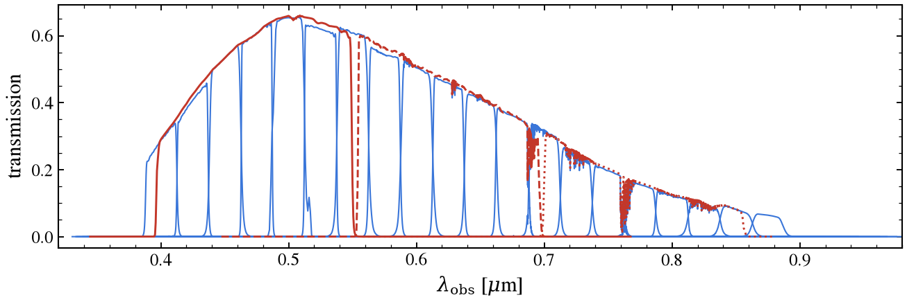
Peak transmission runs 0.34 at m400 to 0.66 near 500 nm to 0.07 at m875. This envelope is the quantum efficiency, which cancels in AB photometry (where only the shape of \(T\) enters). It would matter for absolute count rates.
Prediction
[7]:
SSP_NAME = "prsc_miles_chabrier_wNE"
ssp = tengri.load_ssp(SSP_NAME, download=True)
obs = Observation(photometry=Photometry.from_names(FILTERS))

sed_model = SEDModel.build(
    ssp_data=ssp,
    observation=obs,
    approx=WavePrecomp(),
    sfh=builders.sfh.tsnorm(all_params=FREE),
    dust_attenuation=builders.dust.two_component(
        all_params=Fixed(DEFAULT), law="calzetti", tau_diff=Uniform(0.0, 1.0)
    ),
    dust_emission=builders.dust.emission.modified_blackbody(all_params=Fixed(DEFAULT)),
    neb={"type": "ssp"},
    met={"logzsol": Uniform(-1.5, 0.3)},
    redshift=Fixed(0.0062),
)
forward = ForwardModel.build(sed=sed_model)
print(f"free parameters ({sed_model.spec.n_free}): {', '.join(sed_model.spec.free_params)}")
free parameters (7): dust_tau_diff, met_logzsol, sfh_tsnorm_log_total_mass, sfh_tsnorm_peak_lbt_gyr, sfh_tsnorm_skew, sfh_tsnorm_trunc, sfh_tsnorm_width_gyr
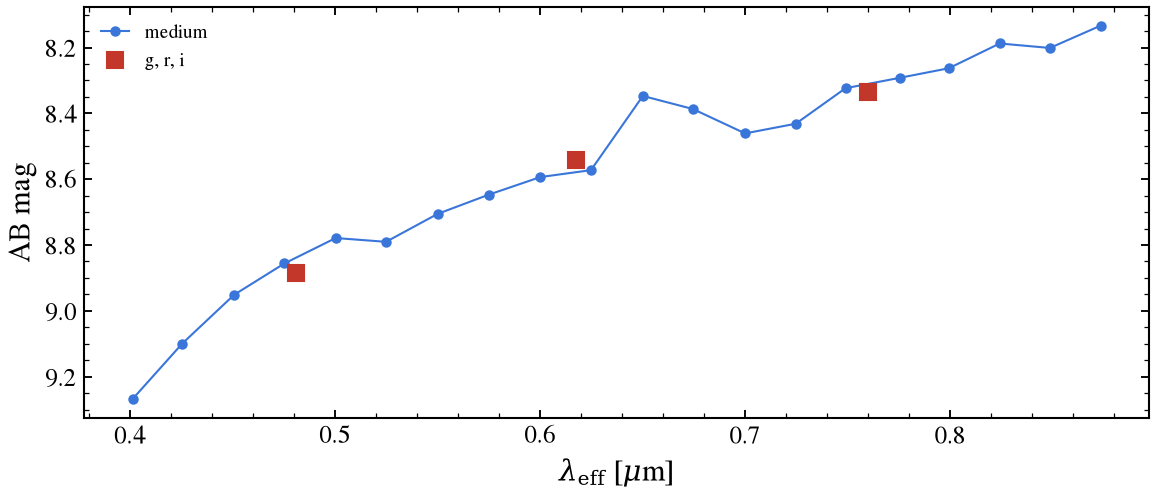
predict_photometry returns one flux per band in the order named. This is the surface the likelihood calls.
[8]:
key_truth, key_mock, key_fit = jax.random.split(jax.random.PRNGKey(11), 3)
truth = sed_model.spec.sample(key_truth)

fnu_pred = np.asarray(sed_model.predict_photometry(truth))
mag_pred = -2.5 * np.log10(fnu_pred) - 48.60
wave_um = effective_wavelengths_um(obs.photometry)

n_med = len(BANDS_MEDIUM)
fig, ax = plt.subplots(figsize=(8.0, 3.6))
ax.plot(wave_um[:n_med], mag_pred[:n_med], "o-", ms=4, lw=1.0, color=C_MODEL, label="medium")
ax.plot(wave_um[n_med:], mag_pred[n_med:], "s", ms=8, color=C_DATA, label="g, r, i")
ax.invert_yaxis()
ax.set(xlabel=r"$\lambda_{\rm eff}$ [$\mu$m]", ylabel="AB mag")
ax.legend(frameon=False, fontsize=9)
fig.tight_layout()
Fit
ADU and a zeropoint reach an ingestible unit in one step:
There is no ADU flux_unit because a zeropoint is calibration, not a unit. The counts below come from the model above, so the fit can be compared to the truth.
[9]:
ZP = dict.fromkeys(FILTERS, 23.89)  # per band in practice, near-identical here

mock = generate_mock(sed_model, truth, key=key_mock, snr=30.0)
fnu = np.asarray(mock["flux_obs"])
sigma = np.asarray(mock["noise"])

mag = -2.5 * np.log10(fnu) - 48.60
adu = 10.0 ** (-0.4 * (mag - np.array([ZP[b] for b in FILTERS])))
adu_err = adu * np.log(10.0) / 2.5 * (1.0857 * sigma / fnu)
print(f"ADU range: {adu.min():.0f} - {adu.max():.0f}")
ADU range: 670895 - 2077551
ingest_catalog takes the column names as they are, and the redshift column explicitly.
[10]:
mag_obs = np.array([ZP[b] for b in FILTERS]) - 2.5 * np.log10(adu)
mag_err = 1.0857 * adu_err / adu

table = {"redshift": np.array([0.0062])}
for j, band in enumerate(FILTERS):
    table[f"flux_{band}"] = np.array([mag_obs[j]])
    table[f"err_{band}"] = np.array([mag_err[j]])

arrays = ingest_catalog(
    table,
    photometry=obs.photometry,
    flux_unit="ab_mag",
    flux_cols=[f"flux_{b}" for b in FILTERS],
    err_cols=[f"err_{b}" for b in FILTERS],
    redshift_col="redshift",
)
print(f"round trip max |dF/F|: {np.abs(arrays.flux[0] / fnu - 1.0).max():.2e}")
round trip max |dF/F|: 1.07e-14
Zeropoint uncertainty is often already inside a delivered error column, so adding NoiseModel(calibration_floor=...) on top counts it twice. Zeropoint uncertainty is also shared across every source in a band rather than drawn per source, which no per-fit floor represents. This matters when sources are fitted jointly or read as a trend.
[11]:
t0 = perf_counter()
posterior = forward.fit(arrays.flux[0], arrays.noise[0], key=key_fit, verbose=False)
print(f"Posterior fit: {perf_counter() - t0:.1f} s")

print(f"\n{'parameter':<20}{'truth':>12}{'p16':>12}{'p50':>12}{'p84':>12}")
print("-" * 68)
for pname in sed_model.spec.free_params:
    samples = np.asarray(posterior.samples[pname])
    p16, p50, p84 = np.percentile(samples, [16, 50, 84])
    true_val = float(truth[pname])
    print(f"{pname:<20}{true_val:>12.3f}{p16:>12.3f}{p50:>12.3f}{p84:>12.3f}")
Posterior fit: 11.6 s

parameter                  truth         p16         p50         p84
--------------------------------------------------------------------
dust_tau_diff              0.188       0.082       0.197       0.332
met_logzsol                0.092      -0.191       0.036       0.208
sfh_tsnorm_log_total_mass      11.432      11.405      11.484      11.549
sfh_tsnorm_peak_lbt_gyr       3.760       1.771       5.171       9.270
sfh_tsnorm_skew            0.389      -0.041       0.601       0.859
sfh_tsnorm_trunc           6.061       2.540       5.632       8.487
sfh_tsnorm_width_gyr       2.732       1.755       3.246       4.433
The stellar mass returns to within 0.07 dex; the shape of the star-formation history, the metallicity and the dust optical depth stay broad. Twenty-three optical bands with no ultraviolet or infrared coverage cannot separate them. For many sources, fit them as a Catalog (notebook 11).