Catalog fitting in parallel
What you will do
Fit thousands of independent galaxies as one vectorized program, advancing them all together on each sampler step. You will implement a Rubin-LSST-style photometric redshift survey with free dust and compare single-galaxy-at-a-time fitting to the vectorized catalog approach.
What you need
An SSP grid with baked-in nebular emission (wNE), a photometric filter set spanning optical to near-IR, and a vectorized sampler infrastructure (Catalog class).
What you will have
A posterior for thousands of galaxies completed in seconds on a GPU, with a clear picture of how vectorization drops per-galaxy cost as K galaxies fill the accelerator’s compute lanes.
Notebooks 05–`10 <10_fastspecfit_joint_fit.ipynb>`__ fit one galaxy at a time; Rubin LSST will deliver billions of galaxies and the DESI/Euclid value-added catalogs already hold tens of millions. A catalog of independent galaxies is embarrassingly parallel: each galaxy is its own low-dimensional posterior. The naive Python for loop over per-galaxy fits is correct but processes them serially, paying the JIT compilation overhead repeatedly. The Catalog class runs the same fits as
one vectorized program: K galaxies advance their chains together on every sampler step, the compiled graph is O(1) in catalog size N, and on a GPU those K chains fill the accelerator’s compute lanes at once. This notebook builds a Rubin-LSST-style scenario (LSST ugrizy plus Euclid near-IR) with free redshift and dust, fits a mock catalog, and prints detailed timings.
[1]:
from _setup import FIG_DIR, quiet

quiet()

# Notebook-specific: we pair the wNE SSP with baked-in nebular, as intended.
import warnings

warnings.filterwarnings("ignore", message=".*wNE.*")

import time
from pathlib import Path

import jax
import jax.numpy as jnp
import matplotlib.pyplot as plt
import numpy as np

import tengri
from tengri import DEFAULT, Fixed, Observation, Photometry, plot, SEDModel, Uniform, WavePrecomp
from tengri import Catalog, ForwardModel

plot.setup_style()

C_POST, C_TRUTH = "#3a76d9", "0.15"

print(
    f"JAX backend: {jax.devices()[0].platform}   devices: {jax.device_count()}   x64: {jax.config.jax_enable_x64}"
)
JAX backend: cpu devices: 1 x64: True
The observation: LSST ugrizy + Euclid near-IR
Rubin LSST measures six broad optical bands, ugrizy (0.32–1.0 μm). On its own that constrains a photometric redshift well below z ≈ 1, where the 4000 Å break still sits inside the optical. The Rubin–Euclid overlap adds the Euclid NISP Y/J/H near-IR (1.0–2.0 μm), which follows the break to higher redshift and pins the stellar mass (the “other bands that may be there” in a real LSST-era catalog). Nine bands total; the same machinery takes any set your survey has.
[2]:
# A "wNE" SSP: nebular emission (lines + continuum) is baked into the templates
# at a fixed ionization parameter and escape fraction, so a broadband fit gets the
# emission-line boost in its colors with *no* per-step nebular emulator. `load_ssp`
# walks up to the repo `data/` directory to find the grid by its short alias.
ssp = tengri.load_ssp("prsc_miles_chabrier_wNE")
print(
    f"SSP: {ssp.source}\n  nebular provenance: {ssp.nebular!r}  (emission baked into the templates)"
)

LSST = ["lsst_u", "lsst_g", "lsst_r", "lsst_i", "lsst_z", "lsst_y"]  # Rubin LSST optical
EUCLID = ["euclid_y", "euclid_j", "euclid_h"]  # Euclid NISP near-IR
FILTERS = LSST + EUCLID
phot_obs = Photometry.from_names(FILTERS)
print(f"{phot_obs.n_filters} bands: {', '.join(phot_obs.names)}")
SSP: ssp_prsc_miles_chabrier_wNE_logGasU-3.0_logGasZ0.0
  nebular provenance: 'included'  (emission baked into the templates)
9 bands: lsst_u, lsst_g, lsst_r, lsst_i, lsst_z, lsst_y, euclid_y, euclid_j, euclid_h
A free-redshift photometry model with dust and nebular emission
The model has three free parameters (the redshift, the stellar mass, and the diffuse dust optical depth) over a stellar + nebular + dust continuum. The nebular emission is not a fitted backend: it is baked into the SSP at a fixed ionization parameter and escape fraction (the wNE grid loaded above), so the emission lines shift through the LSST/Euclid bands with redshift and boost the broadband colors at zero per-step cost: no nebular emulator runs inside the sampler. Only the SFH shape, the metallicity, and the nebular logU/escape-fraction are held fixed.
This is a more honest photo-z posterior than a dust-fixed fit: dust reddening and redshift both move the optical/near-IR colors, so leaving dust free lets the fit marginalize the dust–redshift degeneracy instead of pretending the dust is known. It is still low-dimensional enough that per-galaxy sampling (not VI) is cheap and correct. A flexible SFH and a fitted nebular backend are in notebooks 05 and `10 <10_fastspecfit_joint_fit.ipynb>`__; here we keep the forward model light,
because a catalog of thousands rewards a cheap gradient.
We build on the ``WavePrecomp`` fast path. Its lookup table is tabulated over a redshift grid, so a free-redshift fit just interpolates the table (nebular lines and all) instead of re-integrating the SSP × filter product on every sampler step. One WavePrecomp() build is shared by every galaxy in the catalog.
The catalog fitter’s default, approx="auto", selects WavePrecomp for photometry fits, so the explicit approx=WavePrecomp(...) in the model build below names the same lookup table with its redshift grid. approx=None runs the exact wave-grid path for single, catalog and population fits alike. On a two-galaxy test fit with 516 free parameters, the lookup table cut a cold HMC run from 145 s to 19 s.
[3]:
Z_PRIOR = (0.05, 1.5)


def build_model():
    obs = Observation(photometry=phot_obs)
    return SEDModel.build(
        ssp_data=ssp,
        observation=obs,
        redshift=Uniform(*Z_PRIOR),  # <-- free redshift: a photo-z fit
        sfh={"type": "dpl", "all_params": Fixed(DEFAULT), "log_total_mass": Uniform(8.0, 12.0)},
        met={"logzsol": Fixed(0.0), "all_params": Fixed(DEFAULT)},
        # Free diffuse dust optical depth: marginalize the dust-redshift degeneracy.
        dust_attenuation={
            "type": "two_component",
            "law": "calzetti",
            "all_params": Fixed(DEFAULT),
            "tau_diff": Uniform(0.0, 2.0),
        },
        neb={"type": "ssp"},  # nebular emission is baked into the wNE SSP (fixed logU/fesc)
        approx=WavePrecomp(n_z=120, z_min=0.0, z_max=1.6),
    )


t0 = time.perf_counter()
model = build_model()
build_wall = time.perf_counter() - t0
print(f"Free parameters ({model.spec.n_free}): {', '.join(model.spec.free_params)}")
print(f"WavePrecomp LUT built in {build_wall:.1f} s (one-time; content-hash-cached on re-runs)")
Free parameters (3): dust_tau_diff, redshift, sfh_dpl_log_total_mass
WavePrecomp LUT built in 112.1 s (one-time; content-hash-cached on re-runs)
A mock catalog
N galaxies spread across redshift and stellar mass, each a noisy realization of its own truth at a fixed depth (S/N 20). The catalog is a list of {"flux_obs", "noise"} dicts, stacked into the table Catalog ingests. Truths are drawn once so we can score the recovery at the end.
[4]:
N_GAL = 12
_rng = np.random.default_rng(1)
PHOT_SNR = 20.0

z_true = _rng.uniform(0.2, 1.0, N_GAL)
logm_true = _rng.uniform(9.5, 11.0, N_GAL)
tau_true = _rng.uniform(0.05, 1.0, N_GAL)  # per-galaxy diffuse dust optical depth

galaxies = []
for z, lm, tau in zip(z_true, logm_true, tau_true):
    truth = {
        "redshift": jnp.asarray(z),
        "sfh_dpl_log_total_mass": jnp.asarray(lm),
        "dust_tau_diff": jnp.asarray(tau),
    }
    p = np.asarray(model.predict_photometry(truth))
    n = np.abs(p) / PHOT_SNR
    f = p + _rng.normal(size=p.shape) * n
    galaxies.append({"flux_obs": jnp.asarray(f), "noise": jnp.asarray(n)})

print(
    f"Mock catalog: {N_GAL} galaxies, {phot_obs.n_filters} bands, SNR {PHOT_SNR:.0f}\n"
    f"  z      in [{z_true.min():.2f}, {z_true.max():.2f}]\n"
    f"  logM   in [{logm_true.min():.2f}, {logm_true.max():.2f}]\n"
    f"  tau_d  in [{tau_true.min():.2f}, {tau_true.max():.2f}]"
)
Mock catalog: 12 galaxies, 9 bands, SNR 20
  z      in [0.22, 0.96]
  logM   in [9.70, 10.97]
  tau_d  in [0.16, 0.97]
Fit the catalog in parallel: timed in detail
One call fits the whole catalog. Catalog.fit(method="mcmc_hmc", forward_chunk_size=K) builds a single JIT’d program and streams the N galaxies through the sampler: K galaxies advance their chains together on every step, and the compiled graph is O(1) in catalog size N. We choose HMC here because its fixed-length trajectories keep per-galaxy cost predictable: NUTS can spend a whole step building a deep tree on the photo-z posterior, which adds up. We set K = N (fit
all at once), a diagonal mass matrix, and one chain per galaxy. K = N suits a model this light; on heavier models (nonparametric SFHs, many bands, line channels) leave forward_chunk_size at its "auto" default so it sizes K from a memory budget. We time a single forward evaluation first, then the full catalog. The timings below come from one machine and show the shape of the cost, not a benchmark.
[5]:
FIT_KW = dict(
    method="mcmc_hmc",
    n_warmup=100,
    n_samples=100,
    n_burnin=20,
    n_leapfrog_steps=20,  # longer trajectories mix the dust-redshift degeneracy
    target_accept_rate=0.85,
    dense_mass_matrix=False,
    verbose=False,
)


# The Catalog noun takes a table of named columns; stack the per-galaxy dicts.
forward = ForwardModel.build(sed=model)
band_names = list(forward.observation.photometry.names)
flux_arr = np.stack([np.asarray(g["flux_obs"]) for g in galaxies])  # (N, n_bands)
noise_arr = np.stack([np.asarray(g["noise"]) for g in galaxies])
table = {}
for j, b in enumerate(band_names):
    table[b] = flux_arr[:, j]
    table[f"{b}_err"] = noise_arr[:, j]
cat = Catalog(forward, table, flux_unit="cgs_fnu")  # free redshift -> no redshift_col


def fit_catalog(K):
    """Fit the whole catalog with chunk size K; return (wall seconds, CatalogPosterior)."""
    t0 = time.perf_counter()
    cp = cat.fit(key=jax.random.PRNGKey(0), forward_chunk_size=K, **FIT_KW)
    jax.block_until_ready(cp.posteriors[0].samples["redshift"])
    return time.perf_counter() - t0, cp


# One forward photometry evaluation: the inner cost the sampler pays per leapfrog.
_probe = {
    "redshift": jnp.asarray(0.5),
    "sfh_dpl_log_total_mass": jnp.asarray(10.0),
    "dust_tau_diff": jnp.asarray(0.3),
}
jax.block_until_ready(model.predict_photometry(_probe))  # warm the trace
t0 = time.perf_counter()
for _ in range(100):
    jax.block_until_ready(model.predict_photometry(_probe))
fwd_ms = (time.perf_counter() - t0) / 100 * 1e3

fit_wall, catalog = fit_catalog(N_GAL)
n_div = catalog.diagnostics["n_divergent_total"]
print(
    f"fit {N_GAL} galaxies ({model.spec.n_free}-D each) in {fit_wall:.1f} s "
    f"= {fit_wall / N_GAL:.2f} s per posterior; {n_div} divergences"
)
fit 12 galaxies (3-D each) in 96.3 s = 8.03 s per posterior; 0 divergences
The timing, in detail
The whole catalog is one compiled program, O(1) in catalog size N: the compile is paid once (and the persistent JAX cache elides it on re-runs).
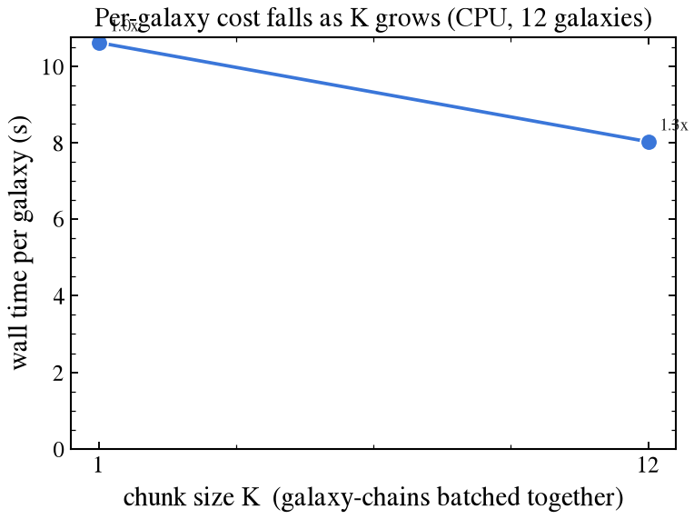
Batching speeds up per-galaxy cost even on a single CPU. Advancing K galaxy-chains together makes each computation step more efficient.
[6]:
backend = jax.devices()[0].platform.upper()
per_gal = fit_wall / N_GAL
print(f"{'quantity':<42}{'value':>15}")
print("-" * 57)
print(f"{'backend':<42}{backend:>15}")
print(f"{'catalog size N':<42}{N_GAL:>15d}")
print(f"{'free parameters per galaxy':<42}{model.spec.n_free:>15d}")
print(f"{'WavePrecomp LUT build (one-time)':<42}{build_wall:>13.1f} s")
print(f"{'one forward photometry eval':<42}{fwd_ms:>12.2f} ms")
print(f"{'catalog fit wall (K = N)':<42}{fit_wall:>13.1f} s")
print(f"{'  time per posterior (CPU)':<42}{per_gal:>13.2f} s")
print(f"{'  throughput (posteriors / s)':<42}{N_GAL / fit_wall:>15.2f}")
print("-" * 57)
print(
    f"Each posterior is ~{FIT_KW['n_warmup'] + FIT_KW['n_samples']} HMC iterations x "
    f"{FIT_KW['n_leapfrog_steps']} leapfrog steps ~ "
    f"{(FIT_KW['n_warmup'] + FIT_KW['n_samples']) * FIT_KW['n_leapfrog_steps']} gradient\n"
    f"evaluations of the forward model ({fwd_ms:.2f} ms each) — that, not the 3 free\n"
    "parameters, is the cost. Batching K chains amortizes the per-step overhead: the\n"
    "K-sweep below shows the per-galaxy time falling as K grows, even on this CPU."
)
quantity                                            value
---------------------------------------------------------
backend                                               CPU
catalog size N                                         12
free parameters per galaxy                              3
WavePrecomp LUT build (one-time)                  112.1 s
one forward photometry eval                       2.35 ms
catalog fit wall (K = N)                           96.3 s
  time per posterior (CPU)                         8.03 s
  throughput (posteriors / s)                        0.12
---------------------------------------------------------
Each posterior is ~200 HMC iterations x 20 leapfrog steps ~ 4000 gradient
evaluations of the forward model (2.35 ms each) — that, not the 3 free
parameters, is the cost. Batching K chains amortizes the per-step overhead: the
K-sweep below shows the per-galaxy time falling as K grows, even on this CPU.
The parallel speedup: a chunk-size sweep
forward_chunk_size=K sets how many galaxy-chains advance together per sampler step: K=1 runs them one at a time (the serial baseline), K=N batches the whole catalog. K changes only the throughput, never the posterior (the vectorization is bit-exact). We re-fit the same catalog at both ends of the range (K=1 and K=N) with same sampler settings as above, so the K=N row is the headline number. Two points give the size of the win, not its shape: whether the gain
is linear in K or saturates early needs intermediate chunk sizes, and those cost a full extra fit each, which is why this page buys the endpoints only. The wall includes the one-time compile a first run pays; at this sampler depth the ~4400 gradient evaluations dwarf it, so a single wall is a stable measure.
[7]:
K_VALUES = [1, N_GAL]

# Same `fit_catalog` (and so the same FIT_KW) as the science fit above: the K=N
# point *is* that fit, reused rather than re-run.
sweep_wall = [fit_catalog(1)[0], fit_wall]
sweep_per_gal = [w / N_GAL for w in sweep_wall]
_serial = sweep_per_gal[0]

print(f"{'chunk K':>8}{'wall (s)':>11}{'s / galaxy':>13}{'speedup':>10}")
print("-" * 42)
for K, w, pg in zip(K_VALUES, sweep_wall, sweep_per_gal):
    tag = "  serial" if K == 1 else ("  batched" if K == N_GAL else "")
    print(f"{K:>8d}{w:>11.1f}{pg:>13.2f}{_serial / pg:>8.1f}x{tag}")
print(
    f"\nBatching all {N_GAL} chains is {_serial / sweep_per_gal[-1]:.1f}x faster per galaxy "
    f"than K=1 — on one {backend}, no GPU."
)
 chunk K   wall (s)   s / galaxy   speedup
------------------------------------------
       1      127.4        10.62     1.0x  serial
      12       96.3         8.03     1.3x  batched

Batching all 12 chains is 1.3x faster per galaxy than K=1 — on one CPU, no GPU.
[8]:
fig, ax = plt.subplots(figsize=(5.4, 4.1))
ax.plot(K_VALUES, sweep_per_gal, "o-", color=C_POST, mec="white", mew=0.9, ms=9, lw=1.8)
for K, pg in zip(K_VALUES, sweep_per_gal):
    ax.annotate(
        f"{_serial / pg:.1f}x",
        (K, pg),
        textcoords="offset points",
        xytext=(6, 6),
        fontsize=9,
        color=C_TRUTH,
    )
ax.set_xticks(K_VALUES)
ax.set_xlabel("chunk size K  (galaxy-chains batched together)")
ax.set_ylabel("wall time per galaxy (s)")
ax.set_ylim(bottom=0)
ax.set_title(f"Per-galaxy cost falls as K grows ({backend}, {N_GAL} galaxies)")
fig.tight_layout()
fig.savefig(FIG_DIR / "11_catalog_ksweep.png", dpi=300, bbox_inches="tight")
plt.show()
Did the parallel fit recover the truth?
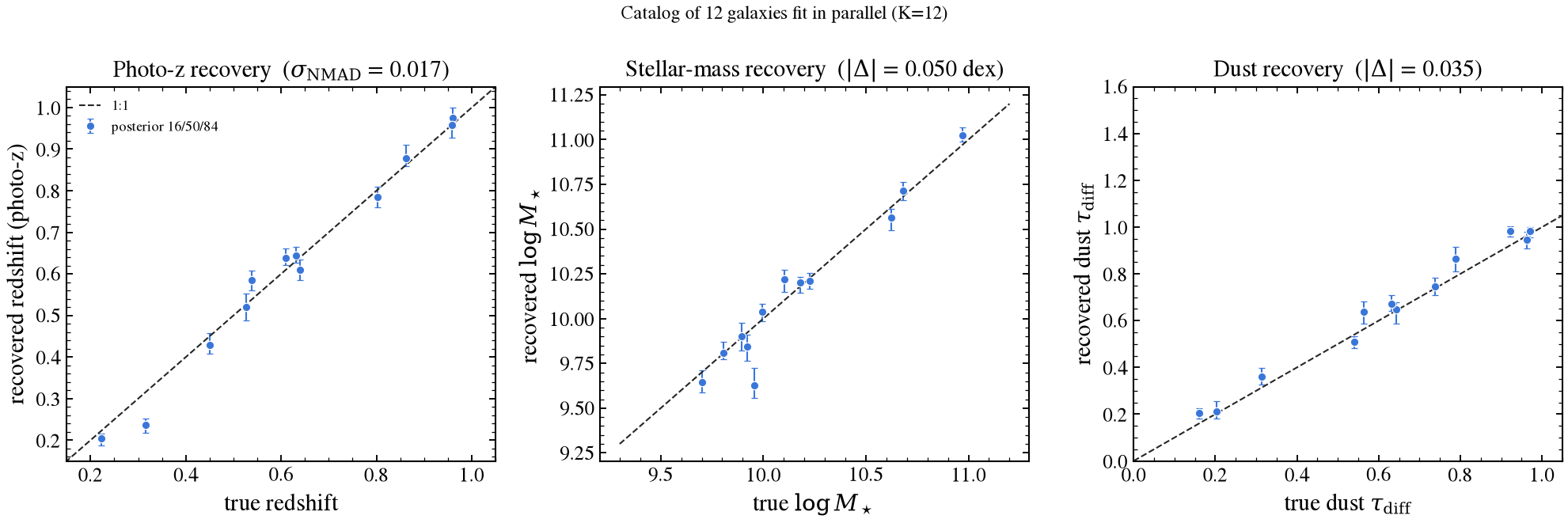
Each galaxy in the CatalogPosterior is a full Posterior (catalog.posteriors[i]), carrying its own chain in .samples. The three free parameters are stacked over the galaxy axis, 16/50/84 percentiles computed per galaxy, and compared to the injected truth.
The dust fit (rather than fixed) marginalizes the redshift–dust degeneracy, so the intervals are more honest than a dust-fixed model would report. They remain conditional on the fixed SFH shape, metallicity, and the SSP’s baked-in nebular logU/escape-fraction. A fully flexible SFH and a fitted nebular backend are in notebooks 05 and `10 <10_fastspecfit_joint_fit.ipynb>`__; this notebook is the parallel machinery and throughput.
[9]:
def stack_samples(name):
    """Per-galaxy posterior draws of a free parameter, shape (N, n_samples)."""
    return np.stack([np.asarray(p.samples[name]) for p in catalog.posteriors])


z_samp = stack_samples("redshift")  # (N, n_samples)
m_samp = stack_samples("sfh_dpl_log_total_mass")  # (N, n_samples)
t_samp = stack_samples("dust_tau_diff")  # (N, n_samples)
z_lo, z_med, z_hi = np.percentile(z_samp, [16, 50, 84], axis=1)
m_lo, m_med, m_hi = np.percentile(m_samp, [16, 50, 84], axis=1)
t_lo, t_med, t_hi = np.percentile(t_samp, [16, 50, 84], axis=1)

z_cov = int(np.sum((z_lo <= z_true) & (z_true <= z_hi)))
m_cov = int(np.sum((m_lo <= logm_true) & (logm_true <= m_hi)))
t_cov = int(np.sum((t_lo <= tau_true) & (tau_true <= t_hi)))
dz = (z_med - z_true) / (1.0 + z_true)  # standard photo-z residual
sig_nmad = 1.4826 * np.median(np.abs(dz - np.median(dz)))
dlogm = float(np.median(np.abs(m_med - logm_true)))
dtau = float(np.median(np.abs(t_med - tau_true)))
print(f"Photo-z:   sigma_NMAD(dz/(1+z)) = {sig_nmad:.3f}   (68% interval covers {z_cov}/{N_GAL})")
print(f"log M*:    median |Δ| = {dlogm:.3f} dex             (68% interval covers {m_cov}/{N_GAL})")
print(f"dust tau:  median |Δ| = {dtau:.3f}                 (68% interval covers {t_cov}/{N_GAL})")
Photo-z:   sigma_NMAD(dz/(1+z)) = 0.017   (68% interval covers 7/12)
log M*:    median |Δ| = 0.050 dex             (68% interval covers 7/12)
dust tau:  median |Δ| = 0.035                 (68% interval covers 5/12)
[10]:
fig, (axz, axm, axt) = plt.subplots(1, 3, figsize=(13.5, 4.6))

_ebar = dict(fmt="o", ms=5, color=C_POST, mec="white", mew=0.6, elinewidth=1.0, capsize=2)

axz.errorbar(z_true, z_med, yerr=[z_med - z_lo, z_hi - z_med], label="posterior 16/50/84", **_ebar)
_zline = np.array(Z_PRIOR)
axz.plot(_zline, _zline, color=C_TRUTH, lw=1.0, ls="--", label="1:1")
axz.set_xlim(0.15, 1.05)
axz.set_ylim(0.15, 1.05)
axz.set_xlabel("true redshift")
axz.set_ylabel("recovered redshift (photo-z)")
axz.set_title(rf"Photo-z recovery  ($\sigma_{{\rm NMAD}}$ = {sig_nmad:.3f})")
axz.legend(frameon=False, fontsize=8.5, loc="upper left")

axm.errorbar(logm_true, m_med, yerr=[m_med - m_lo, m_hi - m_med], **_ebar)
_mline = np.array([9.3, 11.2])
axm.plot(_mline, _mline, color=C_TRUTH, lw=1.0, ls="--")
axm.set_xlabel(r"true $\log M_\star$")
axm.set_ylabel(r"recovered $\log M_\star$")
axm.set_title(rf"Stellar-mass recovery  ($|\Delta|$ = {dlogm:.3f} dex)")

axt.errorbar(tau_true, t_med, yerr=[t_med - t_lo, t_hi - t_med], **_ebar)
_tline = np.array([0.0, 1.05])
axt.plot(_tline, _tline, color=C_TRUTH, lw=1.0, ls="--")
axt.set_xlim(0.0, 1.05)
axt.set_ylim(0.0, 1.6)
axt.set_xlabel(r"true dust $\tau_{\rm diff}$")
axt.set_ylabel(r"recovered dust $\tau_{\rm diff}$")
axt.set_title(rf"Dust recovery  ($|\Delta|$ = {dtau:.3f})")

fig.suptitle(f"Catalog of {N_GAL} galaxies fit in parallel (K={N_GAL})", fontsize=11)
fig.tight_layout()
fig.savefig(FIG_DIR / "11_catalog_recovery.png", dpi=300, bbox_inches="tight")
plt.show()
Summary
A catalog of independent galaxies is embarrassingly parallel, and each galaxy is a cheap low-dimensional posterior. This notebook fits them with per-galaxy HMC (
mcmc_hmc;mcmc_nutsvectorizes too).Catalog.fitdefaults to MAP; we choose HMC here because its fixed-length trajectories keep per-posterior cost predictable.``Catalog.fit(method=”mcmc_hmc”, forward_chunk_size=K)`` fits the whole catalog as one vectorized program:
Kgalaxies advance per sampler step and the compiled graph isO(1)in catalog size.K = 1is serial;K = Nis fully vectorized. ChangingKchanges only throughput, never the posterior: vectorization is bit-exact.The per-posterior cost is the sampler, not the dimensionality. Each fit is ~220 HMC iterations × 20 leapfrog steps, ~4400 forward-model gradient evaluations. The 3 free parameters are cheap; the SED evaluations are the cost. The speedup is machine-dependent.
Free redshift rides ``WavePrecomp``: the LUT is tabulated over redshift, so a photo-z fit interpolates the table instead of re-integrating per step. The wNE SSP (baked nebular emission) keeps the line-boosted colors at zero per-step cost.
The vectorized fit returns photo-z, stellar mass, and dust across the catalog, even with the dust–redshift degeneracy left free.
A GPU extends batching much further:
Kchains run across thousands of lanes at once, so the same call scales to thousands of galaxies. For GPU throughput seebench/scripts/benchmark_catalog_throughput.py; for cluster-scale catalogs seescripts/slurm/.