Nonparametric SFH fits to JWST broad and medium bands
⚠️ Experimental. A research demonstration using experimental APIs that may change between releases.
We fit a Prospector-style continuity star-formation history (piecewise-constant SFR in age bins with Student-t priors on log ratios of adjacent bins, following Leja et al. 2019) to JWST NIRCam photometry at \(z = 1.5\), first for one galaxy and then for a small catalog. The physics is standard; this page focuses on the operational aspects. Two settings decide whether the fit is worthwhile: bin edges that follow the redshift, and a sampling trajectory long enough to cross the correlated ratio posterior.
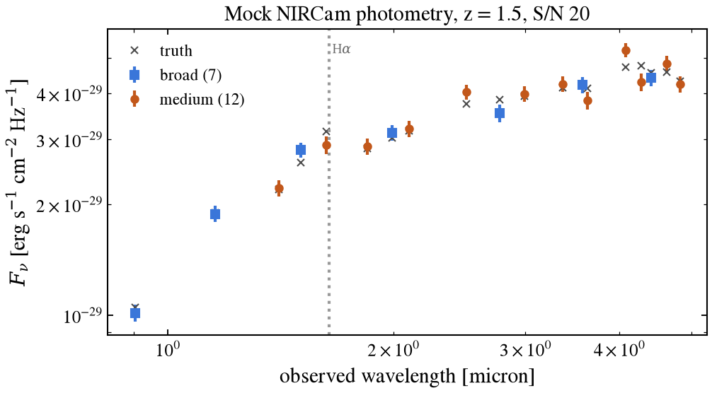
The filter set is 7 broad bands (F090W to F444W) plus 12 medium bands (F140M to F480M). At \(z = 1.5\) the medium bands sample the rest-frame optical continuum whose shape the ratio bins respond to. Since F162M coincides with H\(\alpha\), the fit uses a wNE stellar library with nebular emission baked into the templates.
[1]:
import os
import time
import warnings

# _setup must be imported before jax: it sets TF_CPP_MIN_LOG_LEVEL, which XLA
# only reads at import.
from _plot_style import setup_style
from _setup import FIG_DIR, effective_wavelengths_um, quiet

quiet()
setup_style()

# Four host devices so the default fit's four NUTS chains run in parallel.
os.environ["TENGRI_HOST_DEVICES"] = "4"

# Correct notices, correct to ignore here: the wNE library warns that nebular
# emission is already in the templates and must be paired with the baked-in
# backend, which is the pairing used below; two_component reports the dust
# parameters it holds fixed, and holding them fixed is the point.
warnings.filterwarnings("ignore", message=r"(?s).*is a wNE .*")
warnings.filterwarnings("ignore", message=r"(?s).*run with that physics held constant.*")
# The notice about dense mass matrices and memory is calibrated to heavier models;
# on this fit the peak is a few GB, not the 20+ GB it warns of. The message itself
# is correct and useful as calibrated.
warnings.filterwarnings("ignore", message=r"(?s).*NUTS warmup with dense_mass_matrix.*")

import jax
import matplotlib.pyplot as plt
import numpy as np

import tengri
from tengri import (
    Catalog,
    DEFAULT,
    Fixed,
    ForwardModel,
    FREE,
    Observation,
    Photometry,
    SEDModel,
    Uniform,
    WavePrecomp,
)
from tengri.cosmology import age_at_z
Model
Nine free parameters: total mass plus six bin ratios from the SFH, stellar metallicity, and the diffuse dust optical depth. WavePrecomp routes photometry through a precomputed SSP-by-filter table, which is what makes the samplers below affordable.
The bin edges are tied to the redshift, which is essential. The continuity default is a fixed ladder out to 13.7 Gyr regardless of redshift, while the composite-population kernel excludes star formation older than the universe at the fit redshift. At \(z = 1.5\) the two oldest bins sit outside cosmic time, so they take no likelihood and sample their Student-t prior, though the mass normalization counts them. On this model, a flat history declared at \(\log M = 10.3\) forms 9.80 on
the default ladder (half a dex short). Log-spacing the edges to the age of the universe (as Prospector does) returns 10.30. A SFHBeforeBigBangWarning still fires because the piecewise SFH holds its oldest bin’s rate past the last edge; the shared notebook setup silences it. The normalization is unaffected.
[2]:
Z_GAL = 1.5
SNR = 20.0
N_WARMUP = 1000
N_SAMPLES = 400
N_LEAPFROG = 150

BROAD = [
    "jwst_f090w",
    "jwst_f115w",
    "jwst_f150w",
    "jwst_f200w",
    "jwst_f277w",
    "jwst_f356w",
    "jwst_f444w",
]
MEDIUM = [
    "jwst_f140m",
    "jwst_f162m",
    "jwst_f182m",
    "jwst_f210m",
    "jwst_f250m",
    "jwst_f300m",
    "jwst_f335m",
    "jwst_f360m",
    "jwst_f410m",
    "jwst_f430m",
    "jwst_f460m",
    "jwst_f480m",
]

ssp_data = tengri.load_ssp("prsc_miles_chabrier_wNE")
phot = Photometry.from_names(BROAD + MEDIUM)

# Two youngest edges fixed, the rest log-spaced to the age of the universe.
# Eight edges, so still seven bins and the six ratios the model declares.
T_UNIV = float(age_at_z(Z_GAL))
BIN_EDGES = np.concatenate([[0.0, 0.03], np.logspace(np.log10(0.1), np.log10(T_UNIV), 6)])
print(f"age of universe at z = {Z_GAL}: {T_UNIV:.2f} Gyr")
print("bin edges [Gyr]: " + ", ".join(f"{e:.2f}" for e in BIN_EDGES))

t0 = time.perf_counter()
model = SEDModel.build(
    ssp_data=ssp_data,
    observation=Observation(photometry=phot),
    redshift=Fixed(Z_GAL),
    sfh={"type": "continuity", "all_params": FREE, "bin_edges_gyr": BIN_EDGES},
    # 'all_params': Fixed(DEFAULT) states what the group already does by default. It is
    # here because the disposition is otherwise unstated, which warns: the two
    # remaining metallicity parameters are nuisance knobs this page does not
    # vary, and saying so is what keeps them out of the rendered output.
    met={"logzsol": Uniform(-1.5, 0.3), "all_params": Fixed(DEFAULT)},
    dust_attenuation={
        "type": "two_component",
        "law": "calzetti",
        "all_params": Fixed(DEFAULT),
        # Diffuse screen only, stated rather than inherited. Leaving tau_bc out
        # gave it its declared default of 1.0 -- a frozen magnitude of extra
        # attenuation on every young population, which trades against recent SFR
        # and so is not a neutral nuisance pin in an SFH-recovery fit.
        "tau_bc": 0.0,
        "tau_diff": Uniform(0.0, 2.0),
    },
    neb={"type": "ssp"},
    approx=WavePrecomp(),
)
build_wall = time.perf_counter() - t0

MASS_KEY = next(k for k in model.spec.free_params if k.endswith("log_total_mass"))
RATIO_KEYS = [p for p in model.spec.free_params if "ratio" in p]
print(f"build + WavePrecomp table: {build_wall:.1f} s")
print(f"free parameters ({model.spec.n_free}): {', '.join(model.spec.free_params)}")
age of universe at z = 1.5: 4.28 Gyr
bin edges [Gyr]: 0.00, 0.03, 0.10, 0.21, 0.45, 0.95, 2.02, 4.28
build + WavePrecomp table: 0.9 s
free parameters (9): dust_tau_diff, met_logzsol, sfh_cont_log_total_mass, sfh_cont_ratio_0, sfh_cont_ratio_1, sfh_cont_ratio_2, sfh_cont_ratio_3, sfh_cont_ratio_4, sfh_cont_ratio_5
Mock galaxy
The truth has log total mass \(= 10.3\), constant SFR across the bins (all ratios zero), slightly subsolar metallicity, and moderate diffuse dust. Fluxes are perturbed at signal-to-noise ratio (S/N) 20 per band. A positive ratio means the SFR rises toward the present.
[3]:
rng = np.random.default_rng(4)

truth = {}
truth[MASS_KEY] = 10.3
truth["met_logzsol"] = -0.3
truth["dust_tau_diff"] = 0.3
for name in RATIO_KEYS:
    truth[name] = 0.0

flux_true = np.asarray(model.predict_photometry(truth))
noise = np.abs(flux_true) / SNR
flux_obs = flux_true + rng.normal(size=flux_true.shape) * noise

wave_um = effective_wavelengths_um(phot)
fig, ax = plt.subplots(figsize=(7, 4))
sel_b = np.arange(len(BROAD))
sel_m = np.arange(len(BROAD), len(BROAD) + len(MEDIUM))
ax.errorbar(
    wave_um[sel_b],
    flux_obs[sel_b],
    yerr=noise[sel_b],
    fmt="s",
    ms=6,
    color="#3a76d9",
    label="broad (7)",
)
ax.errorbar(
    wave_um[sel_m],
    flux_obs[sel_m],
    yerr=noise[sel_m],
    fmt="o",
    ms=5,
    color="#c2571a",
    label="medium (12)",
)
ax.plot(wave_um, flux_true, "x", ms=5, color="0.3", label="truth")
ax.axvline(6564.61e-4 * (1 + Z_GAL), ls=":", color="0.6")
ax.text(6564.61e-4 * (1 + Z_GAL), ax.get_ylim()[1] * 0.9, r" H$\alpha$", color="0.4", fontsize=9)
ax.set(
    xscale="log",
    yscale="log",
    xlabel="observed wavelength [micron]",
    ylabel=r"$F_\nu$ [erg s$^{-1}$ cm$^{-2}$ Hz$^{-1}$]",
    title=f"Mock NIRCam photometry, z = {Z_GAL}, S/N {SNR:.0f}",
)
ax.legend(frameon=False)
fig.tight_layout()
fig.savefig(FIG_DIR / "jwst_nonparametric_mock.png", dpi=110)
plt.show()
Individual mode
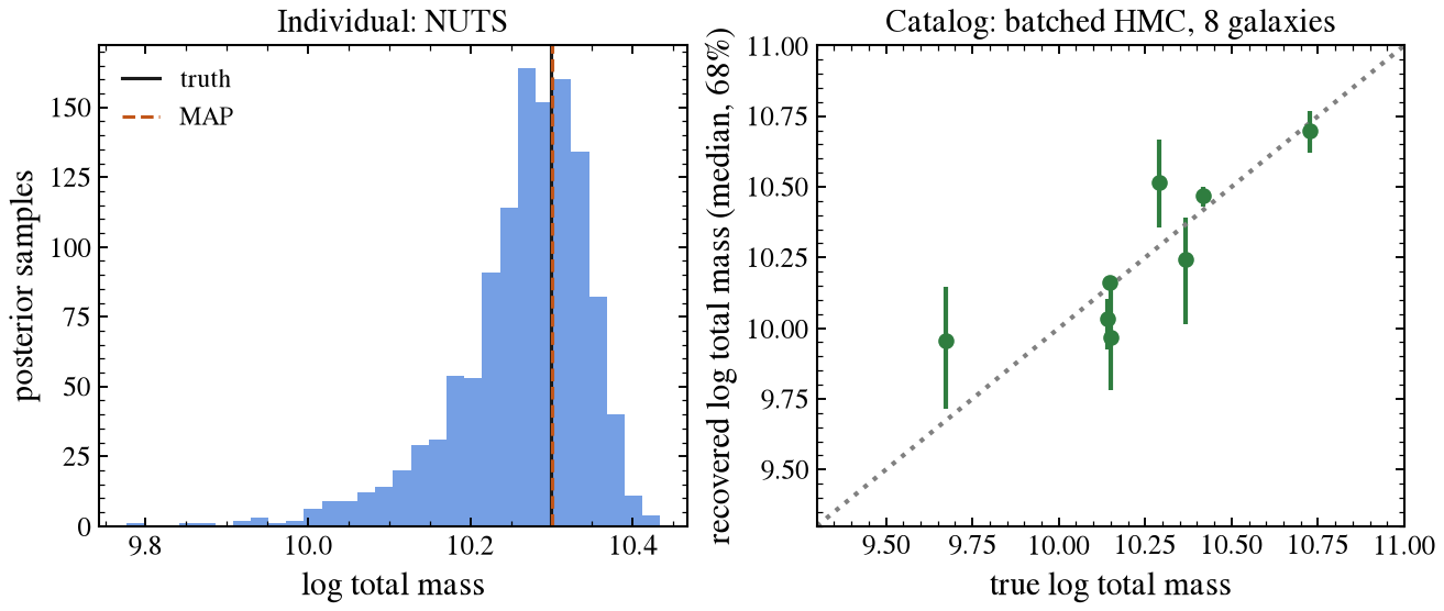
A MAP fit gives the point estimate. The default fit then runs four NUTS chains (150 warmup and 300 draws each), with the stellar mass integrated out analytically, a diagonal metric, and a target acceptance of 0.9. On these correlated bin ratios the dense metric returns far fewer effective samples.
The parameter tau_bc is pinned at 0 here because the NIRCam photometry cannot separate it from the diffuse dust screen; it is part of the posterior geometry the sampler must cross.
[4]:
forward = ForwardModel.build(sed=model)

t0 = time.perf_counter()
map_post = forward.fit(flux_obs, noise, method="map", key=jax.random.PRNGKey(1))
map_wall = time.perf_counter() - t0
map_logm = float(map_post.params[MASS_KEY])
print(f"MAP: {map_wall:.1f} s, log total mass = {map_logm:.2f} (truth {truth[MASS_KEY]:.2f})")

t0 = time.perf_counter()
posterior = forward.fit(
    flux_obs,
    noise,
    key=jax.random.PRNGKey(2),
    verbose=False,
    dense_mass_matrix=False,
    target_accept_rate=0.9,
)
nuts_wall = time.perf_counter() - t0

ess = posterior.effective_sample_size()
ess_name = min(ess, key=ess.get)
ess_val = ess[ess_name]

lo, med, hi = np.percentile(np.asarray(posterior.samples[MASS_KEY]), [16, 50, 84])
print(f"NUTS (4 chains x 300 draws): {nuts_wall:.0f} s, min ESS {ess_val:.0f} ({ess_name})")
print(
    f"log total mass = {med:.2f} [+{hi - med:.2f} -{med - lo:.2f}] (truth {truth[MASS_KEY]:.2f})"
)
  MAP (L-BFGS) complete in 0.1s, 30 iters, 31 evals (converged), loss=18.079580
MAP: 3.1 s, log total mass = 10.30 (truth 10.30)
NUTS (4 chains x 300 draws): 46 s, min ESS 310 (dust_tau_diff)
log total mass = 10.28 [+0.06 -0.09] (truth 10.30)
Catalog mode
We fit eight galaxies at the same redshift, spread over a dex in mass, with their own dust, metallicity, and SFH shape (two rising, two declining, two constant, and two with a burst in the youngest bin). Catalog.fit runs one vectorized program over all of them. The forward_chunk_size is left at its "auto" default, which sizes the batch from a memory budget; forcing K = N on a model this heavy can exceed available RAM.
The catalog runs fixed-length HMC instead of NUTS because a per-step adaptive trajectory length does not vectorize across galaxies. Batched NUTS compiles for many minutes on this model without producing a sample, while fixed-length HMC compiles in seconds. The 150 leapfrog steps cross the correlated ratio posterior. Read the per-galaxy effective sample sizes before trusting any single object. Use the catalog to rank and flag, then refit what matters with the dense-metric posterior above.
[5]:
N_GAL = 8
SHAPES = {
    "rising": np.full(6, 0.4),
    "declining": np.full(6, -0.4),
    "constant": np.zeros(6),
    "burst": np.array([1.3, -0.3, 0.0, 0.0, 0.0, 0.0]),
}
SHAPE_ORDER = ["rising", "declining", "constant", "burst"] * 2

logm_true = rng.uniform(9.5, 10.8, N_GAL)
truths = []
band_names = list(phot.names)
table = {b: np.zeros(N_GAL) for b in band_names}
table.update({f"{b}_err": np.zeros(N_GAL) for b in band_names})
for i in range(N_GAL):
    tr = dict(truth)
    tr[MASS_KEY] = logm_true[i]
    tr["met_logzsol"] = rng.uniform(-0.8, 0.0)
    tr["dust_tau_diff"] = rng.uniform(0.1, 0.8)
    for k, r in zip(RATIO_KEYS, SHAPES[SHAPE_ORDER[i]] + rng.normal(0.0, 0.1, 6)):
        tr[k] = float(r)
    truths.append(tr)
    f_true = np.asarray(model.predict_photometry(tr))
    n = np.abs(f_true) / SNR
    f = f_true + rng.normal(size=f_true.shape) * n
    for j, b in enumerate(band_names):
        table[b][i] = f[j]
        table[f"{b}_err"][i] = n[j]

cat = Catalog(forward, table, flux_unit="cgs_fnu")

t0 = time.perf_counter()
catalog_post = cat.fit(
    key=jax.random.PRNGKey(6),
    method="mcmc_hmc",
    n_warmup=N_WARMUP,
    n_samples=N_SAMPLES,
    n_leapfrog_steps=N_LEAPFROG,
    target_accept_rate=0.9,
    verbose=False,
)
cat_wall = time.perf_counter() - t0

logm_med, logm_lo, logm_hi, ess_per_gal = [], [], [], []
for p in catalog_post:
    s = np.asarray(p.samples[MASS_KEY])
    q16, q50, q84 = np.percentile(s, [16, 50, 84])
    logm_med.append(q50)
    logm_lo.append(q16)
    logm_hi.append(q84)
    ess_per_gal.append(min(p.effective_sample_size().values()))
logm_med, logm_lo, logm_hi = map(np.array, (logm_med, logm_lo, logm_hi))
resid = logm_med - logm_true
print(
    f"catalog HMC: {cat_wall:.1f} s = {cat_wall / N_GAL:.1f} s per galaxy "
    f"({N_GAL} galaxies, one program)"
)
print(f"log total mass recovery: bias {resid.mean():+.2f} dex, scatter {resid.std():.2f} dex")
print(f"min ESS per galaxy: {', '.join(f'{e:.0f}' for e in ess_per_gal)}")
print(f"divergences: {catalog_post.diagnostics.get('n_divergent_total', 'n/a')}")
catalog HMC: 360.1 s = 45.0 s per galaxy (8 galaxies, one program)
log total mass recovery: bias +0.02 dex, scatter 0.15 dex
min ESS per galaxy: 33, 72, 30, 3, 3, 85, 23, 7
divergences: 17
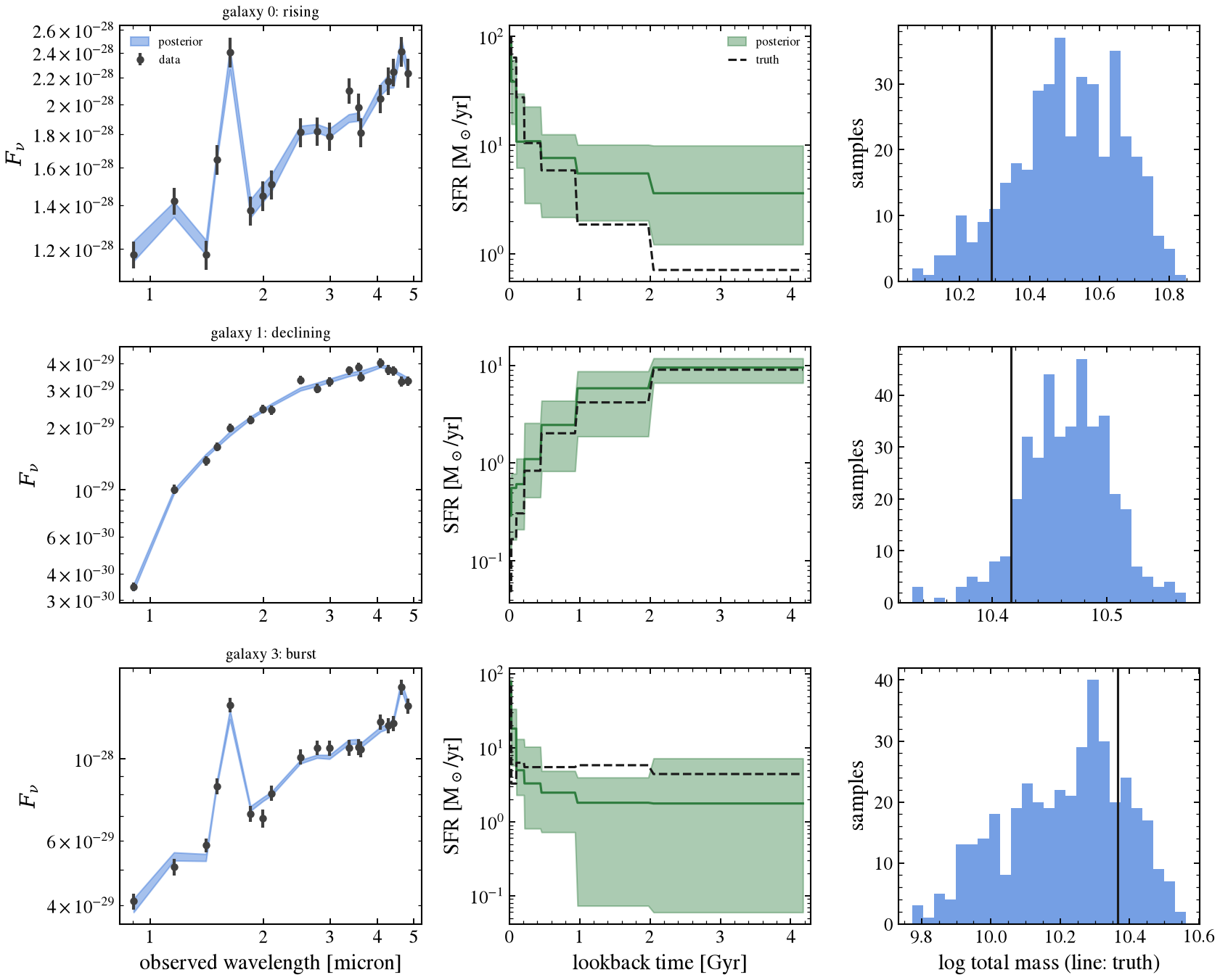
What the catalog fits look like
We show three of the eight (one per SFH shape): the photometry with the posterior model, the recovered history against the input, and the mass posterior. The histories are drawn from the posterior, so the width of the band is the constraint the bands actually place on each age bin. They end at the age of the universe because that is where the composite-population kernel stops counting.
[6]:
N_DRAWS = 40
SHOW = [0, 1, 3]  # rising, declining, burst
ORDER = np.argsort(wave_um)  # band lists are broad-then-medium, not by wavelength


def draw_products(post, key):
    """Model photometry and SFH for N_DRAWS posterior draws."""
    draws = post.resample(key, n=N_DRAWS)
    fluxes, sfrs, lbt = [], [], None
    for i in range(N_DRAWS):
        p = {k: float(v[i]) for k, v in draws.items()}
        fluxes.append(np.asarray(model.predict_photometry(p)))
        s = model.predict_state(p)
        sfrs.append(np.asarray(s.derived["sfr_history"]))
        if lbt is None:
            lbt = np.asarray(s.derived["sfh_grid_lbt_yr"]) / 1e9
    return np.array(fluxes), np.array(sfrs), lbt


fig, axes = plt.subplots(len(SHOW), 3, figsize=(11.5, 3.1 * len(SHOW)))
for row, gal in enumerate(SHOW):
    post = catalog_post[gal]
    fluxes, sfrs, lbt = draw_products(post, jax.random.PRNGKey(20 + gal))
    truth_state = model.predict_state(truths[gal])
    sfr_truth = np.asarray(truth_state.derived["sfr_history"])
    obs = np.array([table[b][gal] for b in band_names])
    err = np.array([table[f"{b}_err"][gal] for b in band_names])

    ax = axes[row, 0]
    ax.errorbar(
        wave_um[ORDER],
        obs[ORDER],
        yerr=err[ORDER],
        fmt="o",
        ms=4,
        color="0.25",
        label="data",
        zorder=3,
    )
    ax.fill_between(
        wave_um[ORDER],
        np.percentile(fluxes, 16, axis=0)[ORDER],
        np.percentile(fluxes, 84, axis=0)[ORDER],
        color="#3a76d9",
        alpha=0.45,
        label="posterior",
    )
    ax.set(xscale="log", yscale="log", ylabel=r"$F_\nu$")
    ax.set_xticks([1, 2, 3, 4, 5])
    ax.set_xticklabels(["1", "2", "3", "4", "5"])
    ax.set_title(f"galaxy {gal}: {SHAPE_ORDER[gal]}", fontsize=10)
    if row == 0:
        ax.legend(frameon=False, fontsize=8)

    ax = axes[row, 1]
    vis = lbt <= T_UNIV  # older than the universe at z: masked by the CSP kernel
    ax.fill_between(
        lbt[vis],
        np.percentile(sfrs, 16, axis=0)[vis],
        np.percentile(sfrs, 84, axis=0)[vis],
        color="#2f7d3f",
        alpha=0.4,
        label="posterior",
    )
    ax.plot(lbt[vis], np.median(sfrs, axis=0)[vis], color="#2f7d3f", lw=1.5)
    ax.plot(lbt[vis], sfr_truth[vis], color="0.1", lw=1.5, ls="--", label="truth")
    ax.set(xlim=(0, T_UNIV), yscale="log", ylabel=r"SFR [M$_\odot$/yr]")
    if row == 0:
        ax.legend(frameon=False, fontsize=8)

    ax = axes[row, 2]
    ax.hist(np.asarray(post.samples[MASS_KEY]).ravel(), bins=25, color="#3a76d9", alpha=0.7)
    ax.axvline(logm_true[gal], color="0.1", lw=1.5)
    ax.set(ylabel="samples")

axes[-1, 0].set_xlabel("observed wavelength [micron]")
axes[-1, 1].set_xlabel("lookback time [Gyr]")
axes[-1, 2].set_xlabel("log total mass (line: truth)")
fig.tight_layout()
fig.savefig(FIG_DIR / "jwst_nonparametric_examples.png", dpi=110)
plt.show()
Recovery
[7]:
fig, (ax1, ax2) = plt.subplots(1, 2, figsize=(9, 4))

ax1.hist(np.asarray(posterior.samples[MASS_KEY]).ravel(), bins=30, color="#3a76d9", alpha=0.7)
ax1.axvline(truth[MASS_KEY], color="0.1", lw=1.5, label="truth")
ax1.axvline(map_logm, color="#c2571a", ls="--", lw=1.5, label="MAP")
ax1.set(xlabel="log total mass", ylabel="posterior samples", title="Individual: NUTS")
ax1.legend(frameon=False)

ax2.errorbar(
    logm_true,
    logm_med,
    yerr=[logm_med - logm_lo, logm_hi - logm_med],
    fmt="o",
    ms=6,
    color="#2f7d3f",
)
lims = [9.3, 11.0]
ax2.plot(lims, lims, ls=":", color="0.5")
ax2.set(
    xlim=lims,
    ylim=lims,
    xlabel="true log total mass",
    ylabel="recovered log total mass (median, 68%)",
    title=f"Catalog: batched HMC, {N_GAL} galaxies",
)

fig.tight_layout()
fig.savefig(FIG_DIR / "jwst_nonparametric_recovery.png", dpi=110)
plt.show()
Cost summary
[8]:
print(f"{'stage':<44}{'wall':>10}")
print("-" * 54)
print(f"{'model build + WavePrecomp (one-time)':<44}{build_wall:>8.1f} s")
print(f"{'MAP, 9 parameters':<44}{map_wall:>8.1f} s")
print(f"{'HMC posterior, single galaxy':<44}{nuts_wall:>8.1f} s")
print(f"{'catalog HMC, per galaxy':<44}{cat_wall / N_GAL:>8.1f} s")
stage                                             wall
------------------------------------------------------
model build + WavePrecomp (one-time)             0.9 s
MAP, 9 parameters                                3.1 s
HMC posterior, single galaxy                    46.4 s
catalog HMC, per galaxy                         45.0 s
These are rules of thumb from this configuration on a laptop CPU with a warm compile cache. MAP takes a second or two. The single-galaxy posterior (printed above as wall time) runs four NUTS chains and returns the full posterior; the catalog runs HMC on each galaxy in the printed seconds per galaxy.
A fit far outside those ranges usually indicates a wrong setting. Check three things, in order: that the bin edges reach the age of the universe at the fit redshift and no further, that the model was built with WavePrecomp, and that the catalog trajectory is long enough. Also check what the sampler did, not just how long it took. A nonparametric fit that returns in seconds has almost certainly not moved, and one that returns a low divergence count alongside a minimum ESS in the single digits
has not moved either. The “Choosing an inference method” page has the sampler decision table.