Known limitations
Tengri is research code under active development (v0.1.0). The forward model and inference pipeline work and are covered by 2000+ tests, but several capabilities are partial. This page collects the caveats you are most likely to encounter.
Verification status
No physics component has completed full external cross-validation against FSPS, Prospector, or CIGALE. The reproduction notebooks under docs/reproduction/ compare specific components against established codes, but the formal verification protocol (docs/dev/verification-protocol.md) lists every major block as still in progress. Do not treat fitted parameters as publication-grade until your component has been cross-validated.
Approximations
Both precompute paths trade a bounded, quantified error for a large speedup. Each does the same thing: integrate everything that does not depend on a free parameter once at build time, then reduce each likelihood call to a small contraction.
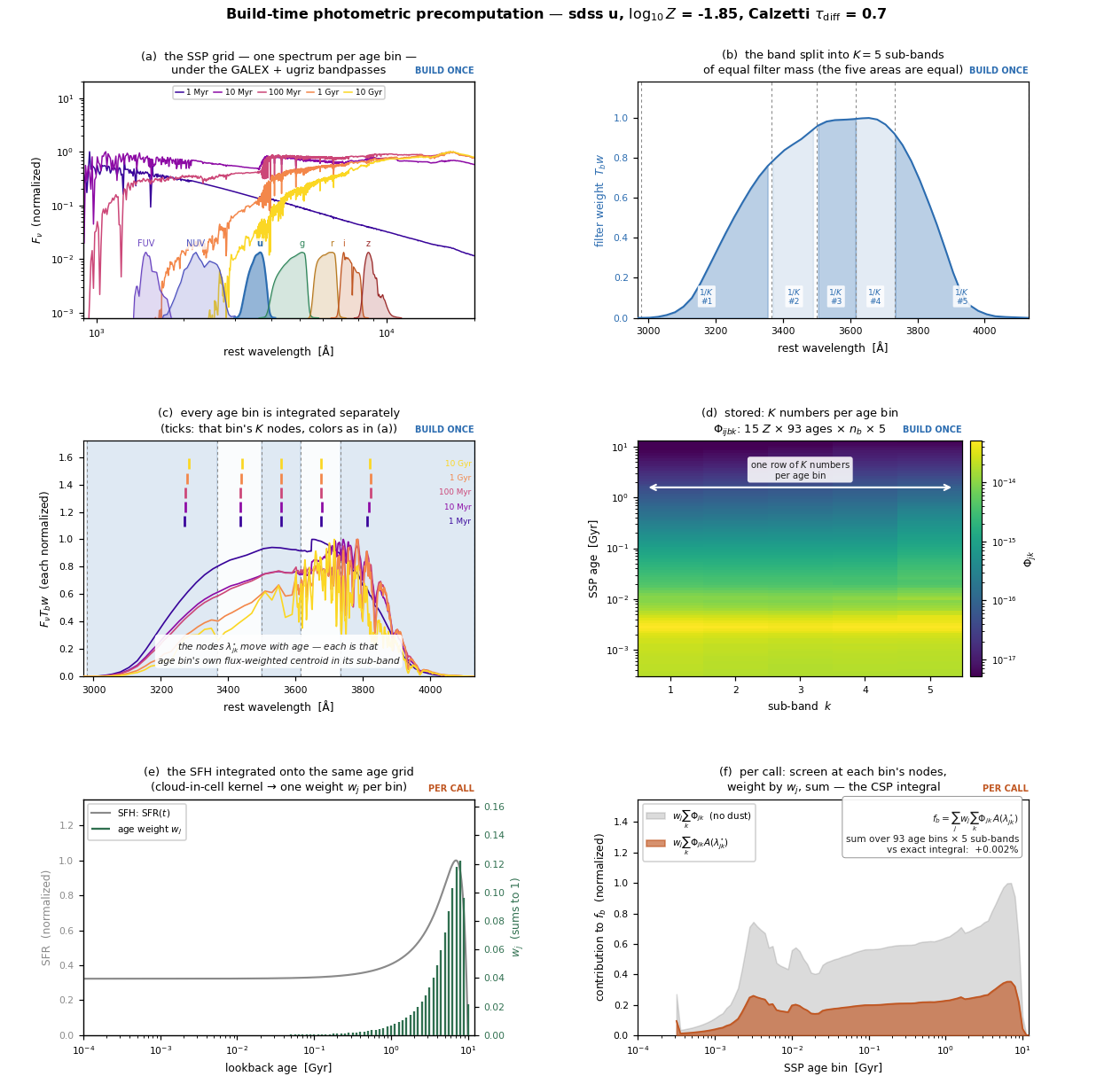
What approx=WavePrecomp() does to a real SSP grid, and where the star
formation history enters. (a) The grid holds one spectrum per age bin;
five are drawn, under the GALEX and ugriz bandpasses. SDSS u is followed
through the rest of the figure. (b) That band is cut into \(K = 5\)
sub-bands of equal filter mass — the five shaded areas are equal, so they
run narrow where the filter is most transmissive and wide out in the wings.
The partition depends on the filter alone. (c) Every age bin is then
integrated separately against that partition, and each gets its own \(K\)
nodes \(\lambda^\star_{jk}\) (the tick rows): a node is that age bin’s own
flux-weighted centroid within its sub-band, so it moves as the spectrum
ages. (d) What is stored is therefore a tensor, not a vector — \(K\)
numbers for every age bin, every metallicity and every band,
\(\Phi_{ijbk}\). None of it depends on a free parameter, so it is all built
once. (e) At fit time the star formation history is integrated onto
that same age grid by the cloud-in-cell kernel, giving one mass weight
\(w_j\) per age bin. (f) The composite-stellar-population flux is then
the double sum \(f_b = \sum_j w_j \sum_k \Phi_{jk} A(\lambda^\star_{jk})\) —
over all 93 age bins and their 5 sub-bands, with the dust screen evaluated
only at the nodes. No wavelength grid is touched at any point in the
likelihood, and for this band the result lands within a few thousandths of
a percent of the exact integral. Generated by
scripts/render_precompute_schematic.py.
The reason a factorization like this needs care: the photometry integral wants \(\langle F_\nu A \rangle_b\) (the SSP spectrum times the dust screen, averaged over the bandpass). Precomputing the two separately would give \(\langle F_\nu \rangle_b \langle A \rangle_b\), and the difference between them is exactly the in-band covariance \(\mathrm{Cov}_b(F_\nu, A)\). That covariance is the entire error term, and the sub-band quadrature buys it back. Additive emitters (dust IR, AGN, radio, X-ray) need none of this: each is a sum of rank-one terms, so it factors through the filter exactly and carries no quadrature error.
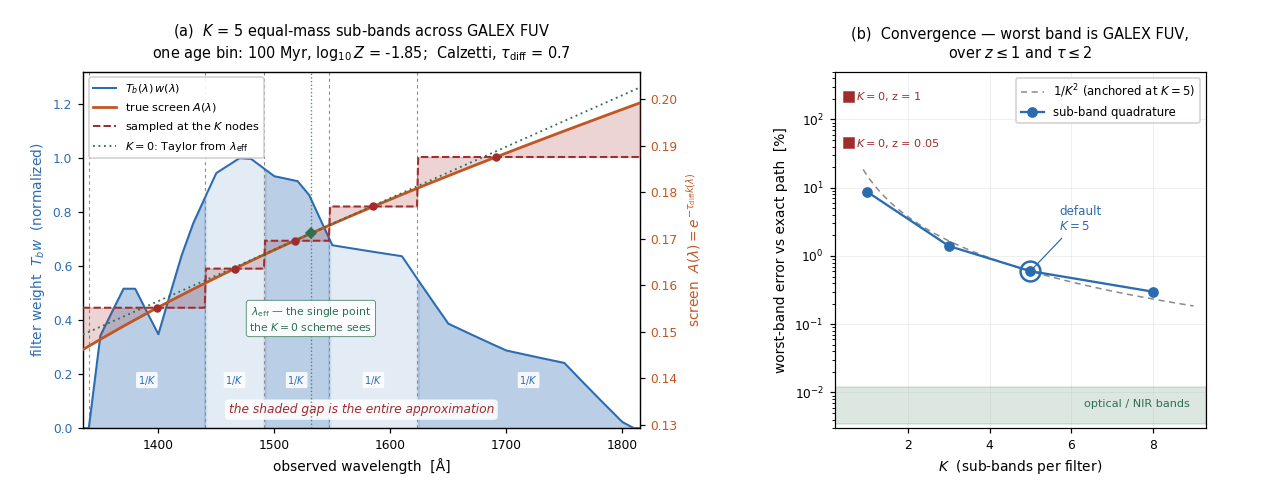
Where the residual error lives. (a) The real GALEX FUV bandpass split
into \(K = 5\) sub-bands of equal filter mass — the five shaded regions have
equal area under \(T_b w\). Each carries one node \(\lambda^\star\), the
template’s own flux-weighted centroid there, so the screen is evaluated at
five points and held constant across each sub-band; the shaded gap between
the true screen and that step function is the whole of the approximation.
Because each node is a first moment, the first moment of the in-band
residual vanishes identically — a first-order correction on top of the
sub-band rule would add exactly zero. Edges and nodes are drawn from the
shipped subband_quadrature partition. Panel (a) is a mild configuration
(\(z = 0\), \(\tau_\mathrm{diff} = 0.7\)) where the \(K = 0\) Taylor extrapolation
still nearly coincides with the true screen; it diverges as redshift and
optical depth grow, which is what the \(K = 0\) points in (b) quantify.
(b) Worst-band error against the exact path over \(z \le 1\) and
\(\tau \le 2\). Generated by scripts/render_precompute_schematic.py.
WavePrecompaccelerates the photometry channel. It precomputes the SSP × filter integrals, with free redshift via interpolation. Each filter is split inton_subbandssub-bands of equal filter mass (default 5), and the multiplicative screens (dust attenuation and IGM transmission) are evaluated at each sub-band’s quadrature node (the template’s own flux-weighted centroid there). Measured against the exact path across GALEX→WISE at z ≤ 1.5 with τ_diff = 0.7 / τ_bc = 1.0, the worst band agrees to ≲0.5%, and the optical/NIR bands to ≲0.01%. Accuracy improves as 1/K²; raiseWavePrecomp(n_subbands=8)for the deep rest-UV. Emission that the quadrature cannot reach (nebular lines, AGN, dust IR) is still projected at the filter’s effective wavelength.WavePrecomp(n_subbands=0)restores the old first-order Taylor projection, which extrapolates the screen from each filter’s effective wavelength instead of evaluating it. That linear-in-λ model is accurate for smooth attenuation curves (optical/IR) but biases rest-UV bands where the curve is steep: at z ≈ 2 with τ ≈ 0.5, SDSS u/g run 5–10% high and GALEX FUV greater than 10× high. A build-timeUserWarningflags such configurations. It is retained only for reproducing results from earlier versions.SpectrumPrecompis the default for spectroscopy fits only where it serves the pixels exactly.approx="auto"takes the spectrum LUT for a spectroscopy fit when three things hold: the pixels are point-sampled or no wider than the model grid (no bin integral),sigma_v_kmsis Fixed, and no banded resolution matrix is attached. Otherwise the fit stays on the exact path, and a freesigma_v_kmssays so once.approx=Nonealways stays exact, and an explicitSpectrumPrecomp()engages the table as before. When the LUT is in use, it applies the same velocity-dispersion and instrument stages as the exact path (σ_v on the model grid, the library-deconvolved instrument kernel on the pixel grid) and agrees with it to better than 1e-3 across the pixels, lines included; with a freesigma_v_kmsthe table broadens the stellar sum per draw on the full model grid, which costs roughly 15 times the exact path per gradient step and warns once, and a banded resolution matrix falls back to the exact path.SpectrumPrecompaccelerates the spectroscopy channel. It precomputes a per-pixel effective-wavelength continuum LUT. It agrees with the exact path to machine precision with zero dust. With dust, it carries the same error class asWavePrecompbut far milder (pixel-wide versus filter-wide): typically ≲1% on the continuum, growing to ~10–15% only in the deep rest-UV at high optical depth. It applies the exact path’s stages in the same order (stellar velocity dispersion on the model grid, IGM, instrument kernel on the pixels) and matches it to better than 2e-3 at every pixel of the line-rich test fixture at R = 2000 and 5000 and \(\sigma_v\) = 300 km/s; a bandedresolution_matrixfalls back to the exact path with a warning. Component coverage: stellar, dust IR, radio, X-ray, AGN, and non-baked nebular (Cue/CloudyGrid) are included in the spectrum LUT. Nebular emission is reddened by the young-limit screen, matching the exact path. BakedIn nebular is carried by the stellar LUT.Joint photometry + spectroscopy is supported under precompute. Either precompute opt-in builds both LUT families, and
approx="auto"puts the spectrum channel on the spectrum LUT under the same three conditions as a spectroscopy fit; the forward pass projects both channels in one fused, cached JIT kernel. For independent per-channel tuning, passapprox=(WavePrecomp(n_z=200), SpectrumPrecomp()). Velocity dispersion and the instrument LSF are applied by the spectrum LUT; with a freesigma_v_kmsthe stellar sum is broadened per draw on the full model grid, which costs roughly an order of magnitude more per gradient step, so a joint fit withapprox=WavePrecomp()keeps a free-sigma_v_kmsspectrum channel on the exact path and says so once. Underapprox="auto"the photometry channel takesWavePrecompand the spectrum channel stays exact when any of the three conditions fails.
Inference backends
Each backend is tagged primary or experimental. Experimental backends
carry explicit [POOR MIXING] or [UNSTABLE] flags (e.g. mcmc_ghmc,
mcmc_mclmc, pathfinder, native_vi_*). Use primary backends for science.
See Choosing an inference method.
Memory
NUTS/VI warmup peaks far above the resident forward model (20+ GB on dense_basis D≈8 with dense_mass_matrix=True). Rules:
Run one NUTS/VI fit per Python process.
On D ≥ 8, use
dense_mass_matrix=Falseormcmc_hmc.WavePrecompkeeps photometry fits in the few-GB range.
Full detail: docs/dev/notebook_orchestration_oom.md.
Physics caveats
The
cb19nebular grid is not shipped.data/cb19_templates.h5is not in the repository, andscripts/download_cb19_templates.pycannot rebuild it because the 3MdB databases hold noCB_19reference (seedocs/internal/advanced/cb19_grid.md). A build that reads the grid raisesFileNotFoundError. Usecloudyorcueuntil the grid is restored.tengri.list_nebular_backends()still listscb19with statusproduction, so do not infer availability from that status.BPASS surviving mass is not metallicity-dependent. No surviving-mass table exists for the BPASS grids (
src/tengri/data/ssp_mass_remaining/PROVENANCE.md). A BPASS build refuses the default source. Passmass_remaining="dsps_fit"to use DSPS’s metallicity-independent fit, which does not track the metallicity dependence of the surviving mass.One filter convention per
Photometry. Every band in aPhotometryobject uses one convention:"bessell"(photon-counting, the default) or"energy"(CIGALE’s energy-type bands such as 2MASS, MIPS, PACS and SPIRE). The two conventions differ by 5 to 40 mmag (about 0.5 to 4 %) depending on band and SED slope. Set the convention to match each detector, and expect that error on bolometer bands if they are measured under the photon-counting convention.AGN torus:
agn/torus.pytoy models are not for science. Useagn_model="skirtor"(Stalevski et al. 2016).Dust IR emission templates must be loaded from
data/; analytic fallbacks are not suitable for science.Dust emission JIT scaling: DL07-family dust-emission models (DL07, DL14, and tabulated variants) build very large JIT graphs when
dust_uminis left free in the sampler. The compiled graph can exceed 2 GB, causing slowdowns (~150× slower) in nested sampling backends. Workarounds: (1) fixdust_uminrather than fitting it, or (2) use fixed-redshift models where the precomputation (approx=WavePrecomp()) amortizes the graph across many calls. Technical details are tracked in the repository’s engineering notes (docs/dev/known_bugs.md on GitHub).Nebular backends:
CueandCloudyGridrequire bare-stellar SSP grids;BakedIncannot varyneb_logU/neb_fesc. Four of sixtengri.recipesneed bare-stellar grids.Metallicity is
log10(Z)absolute on the SSP grid; user-facingneb_logZ_gasislog10(Z/Z_sun).Super-solar metallicity above Z = 0.04 in the PARSEC grids is held at Z = 0.04 for young stars. The Z = 0.06 node of every PARSEC-based grid (
fsps_prsc_*,ssp_prsc_*) has no stars above about 12 Msun for log10(age/yr) <= 7.15, because the PARSEC massive-star tracks stop at Z = 0.04 (Chen et al. 2015). Used as shipped, it is about 800-2700 times low in ionizing photons (Q_H(Z = 0.06) / Q_H(Z = 0.04) = 3.7e-4, 4.1e-4 and 1.3e-3 at log age 5.5, 6.0 and 6.5) and about 16 times low at 1500 A. The loader therefore refuses that part of the node: for log age <= 7.15 a metallicity above Z = 0.04 gives the Z = 0.04 population, and the Z = 0.06 node returns linearly in log age over the next 0.05 dex (one grid step: weight 0 at 7.15, 1 from 7.20), so there is no step in age. Older populations are unchanged. A model warns at build time when its metallicity weights can reach the Z = 0.06 node, that is when themet_logzsolprior’s upper bound plus 3 sigma of the metallicity scatter’s upper bound exceeds the lower edge of that node’s metallicity bin (log10(Z/Z_sun)= 0.544, Z = 0.0497, on the PARSEC grids; 0.572 withtop_z="mist"). Below the edge the node’s weight is exactly zero, so the defaultUniform(-2, 0.2)prior with a scatter of 0.1 dex does not warn. To use a MIST [Z/H] = +0.5 node (FSPS’s zlegend value Z = Z_sun 10^[Z/H] = 0.0449 with Z_sun = 0.0142; MILES, same IMF and ages) at young ages instead, load the grid withtengri.load_ssp(name, top_z="mist"); the node is inserted at that metallicity and the model never extrapolates above it at young ages.top_z="raw"keeps the file as shipped (cross-code comparison with FSPS only). MIST grids are complete at their top node and are not affected.top_z="mist"mixes isochrone sets. Between Z = 0.040 (PARSEC) and 0.0449 (MIST) the young part of the metallicity axis switches isochrone physics, not just metallicity. MIST node / PARSEC Z = 0.04 node, measured onfsps_prsc_miles_chabrierat log age 6.0 / 6.5 / 7.0: Q_H 0.909 / 1.72 / 0.434, L_nu(1500 A) 0.908 / 0.773 / 0.783, V band (mean L_nu over 5000-5900 A) 0.775 / 0.749 / 0.911. A gradient inmet_logzsolover about 0.45-0.50 at young ages reflects that switch. The defaulttop_z="clip"has no such switch.
Reporting
Found something not listed here? Open an issue at https://github.com/suchethac/tengri/issues.