Running tengri on an NVIDIA GPU (CUDA)
This GPU backend is measured, supported, and mostly not worth it for typical use. Unlike the Apple path, nothing here needs a JAX version tengri does not pin: pip install -U "jax[cuda12]" works, and the forward model, gradients, and samplers all run. It works, but for the way most people fit one galaxy at a time it is not faster.
The one-line summary, measured on an RTX 3060 against a 12-core Ryzen 9 5900X:
one galaxy at a time    ->  CPU, by a wide margin. Nothing to amortize.
a wide enough batch     ->  GPU, and the crossover is where to look.
float64 on a GeForce    ->  half the CPU's throughput. The card runs it at 1/64 rate.
float32                 ->  buys nothing on this workload. It is not arithmetic-bound.
The reason is arithmetic intensity, and it is the same reason as on Apple silicon: tengri moves a lot of memory and does very little arithmetic (about 0.12 FLOP per byte on the WavePrecomp path, against the 25–50 FLOP/byte a GPU needs before its ALUs become the limiting factor). That figure is measured in notebooks/apple_mps.py; it is a property of the compiled graph rather than of the device, which is why it predicts both backends. A single galaxy gives the card nothing to do but
wait for memory and the host.
Consumer NVIDIA hardware has a second effect specific to it. GeForce cards run float64 at 1/64 of their float32 rate, so in tengri’s default precision this GPU is slower at dense arithmetic than the CPU beside it:
dense 2048³ matmul |
CPU |
GPU |
|---|---|---|
float32 |
988 GFLOP/s |
10,740 GFLOP/s |
float64 |
379 GFLOP/s |
189 GFLOP/s |
A datacenter card (A100, H100) has roughly a 1/2 rate instead of 1/64, so the float64 row does not transfer. Everything driven by dispatch and memory traffic does.
Two caveats apply to the numbers below.
This GPU was also driving the desktop: Xorg, gnome-shell, and a browser held 1–3 GB and 20–40% utilization throughout. Timings were taken with rotated repetitions and an A/A control, and ratios that do not clear that control are reported as unresolved rather than quoted.
Benchmark one shape per process, since running a forward pass, a gradient, and a fit in one process makes the later ones look worse. The tables come from
bench/scripts/benchmark_device_matrix.py, which spawns a child per cell for that reason.
1. Install and select the device
pip install -U "jax[cuda12]"
No tengri-side changes are required, and you do not need to manage JAX versions. Check what you installed:
import jax; jax.devices() # -> [CudaDevice(id=0)]
Two environment variables matter, and both must be set before Python starts. Setting them after import tengri is too late: constants allocated during the import are already placed on a device and already have a width.
export JAX_PLATFORMS=cuda                    # or cpu, to compare
export XLA_PYTHON_CLIENT_PREALLOCATE=false   # see below
XLA_PYTHON_CLIENT_PREALLOCATE=false is not optional in practice. JAX claims 75% of the card by default, so a second process (a notebook left open or a pytest worker) gets CUDA_ERROR_OUT_OF_MEMORY instead of a device. Pair it with XLA_PYTHON_CLIENT_MEM_FRACTION=0.85 if you want a ceiling rather than growth.
[1]:
import os

# Must precede any import that touches JAX. In a notebook that means the very
# first cell.
os.environ["JAX_PLATFORMS"] = "cuda"
os.environ["XLA_PYTHON_CLIENT_PREALLOCATE"] = "false"
os.environ["TF_CPP_MIN_LOG_LEVEL"] = "2"

import jax
import jax.numpy as jnp
import numpy as np

import tengri

print("device :", jax.devices())
print("x64    :", jax.config.jax_enable_x64)
print("dtype  :", jnp.zeros(1).dtype)
device : [CudaDevice(id=0)]
x64    : True
dtype  : float64
2. Precision is a decision, not a default
CUDA supports both widths, so unlike the Apple backend you have to choose. Tengri defaults to float64 and will hold that choice through its own import. To ask for float32, set it in the environment:
export JAX_ENABLE_X64=0
Tengri honors that and says so once:
JAX_ENABLE_X64=0: tengri is honoring your request for float32 and is NOT
enabling 64-bit precision. Cosmological distances are the known hazard
(d_L^2 at z > 0.01 overflows float32), so any code that forms d_L^2 directly
will produce inf. tengri's own projection avoids it by applying
(1+z)/(4*pi*d_L^2) as a log10 offset, but third-party code may not.
That warning captures the whole float32 story. The forward model carries unrepresentable magnitudes as log10 offsets and comes out correct, while code that forms the linear quantity does not.
Do not use ``SEDModel.build(forward_dtype=”float32”)``. It casts nothing and only emits a DeprecationWarning. The two routes that work are the environment variable above and with jax.enable_x64(False): wrapped around the build and the call.
Load the SSP grid inside the float32 context. A grid loaded while x64 was still on stays float64, and thirteen downstream gates key on wave.dtype, so the fast paths silently never engage and a float32 run quietly measures something else.
If you use float32 on CUDA, turn TF32 off
This issue does not come from tengri, and it is easy to miss. On Ampere and later, XLA lowers float32 matmuls to TF32 by default (19 bits, with a 10-bit mantissa, against float32’s 24). Numerics calibrated on a CPU do not survive that. Tengri’s own float32 Fisher-matrix test fails on CUDA out of the box:
AssertionError: float32 FIM differs from float64 by 3.922e-03 relative
AssertionError: float32 error bars differ from float64 by 4.494e-02
This is a 4% error on parameter error bars; the same test passes on the CPU. Ask for real float32:
export JAX_DEFAULT_MATMUL_PRECISION=highest
Or use jax.config.update("jax_default_matmul_precision", "highest"). Both routes make these tests pass.
``NVIDIA_TF32_OVERRIDE=0`` does not fix it. With that alone the two tests still fail, because XLA selects its own algorithm, so the JAX-level knob is the one that binds.
Setting the matmul precision costs no speed. The batch numbers in section 3 are unchanged to within noise with TF32 disabled (4.42 against 4.45 us per galaxy at batch 2048). Float32’s advantage in tengri comes from moving half as many bytes, not from tensor cores, so there is nothing to trade away.
3. Prediction
We measure one galaxy with five SDSS bands using recipes.mock_recovery_minimal at z = 0.05 (seven free parameters, nebular and AGN off) on the WavePrecomp path that every fit uses.
[2]:
from tengri import SEDModel, WavePrecomp, load_ssp, recipes
from tengri.observation import Observation, Photometry

# load_ssp resolves a short alias and walks parent dirs for data/, so this works
# whatever the working directory is. A cwd-relative data/... path only resolves
# from the repository root, and the notebook executor runs from notebooks/.
ssp = load_ssp("fsps_prsc_miles_chabrier")
obs = Observation(
    photometry=Photometry.from_names(["sdss_u", "sdss_g", "sdss_r", "sdss_i", "sdss_z"])
)
recipe = recipes.mock_recovery_minimal()
recipe["approx"] = WavePrecomp()
model = SEDModel.build(ssp_data=ssp, observation=obs, **recipe)

# For the reference galaxy, we set each free parameter to the median of its declared prior.
# This is not a prior draw (jax.random returns different numbers for the same
# key at float32 and float64, so a sampled fixture compares two different
# galaxies across the precision arms and calls the difference precision error.
params = {
    name: round(
        float(np.asarray(model.spec.get_distribution(name).unstandardize(jnp.zeros(())))), 6
    )
    for name in model.spec.free_params
}
flux = model.predict_photometry(params)
print("photometry [erg/s/cm2/Hz]:", np.asarray(flux))
print("on device                :", flux.devices())
src/tengri/forward/sed_model.py:2869: BakedInNebularWarning: BakedInBackend: nebular emission is baked into the SSP file at a FIXED logU and FIXED escape fraction determined when the SSP grid was generated (commonly logU = −3, but depends on the SSP file). The ionization parameter and escape fraction are NOT free parameters — varying neb_logU or neb_fesc in your Parameters will have no effect. Check your SSP file's nebular assumptions. Switch to CloudyGridBackend or CueBackend to vary nebular properties. To suppress when building via SEDModel.build: warnings.filterwarnings('ignore', message='BakedInBackend: nebular emission is baked'). (ionizing_source_warning='suppress' also works, but it is a BakedInBackend(...) constructor argument and the build grammar does not forward it.)
  self._nebular_backend = BakedInBackend()
photometry [erg/s/cm2/Hz]: [3.59509284e-28 1.29919346e-27 2.29231601e-27 2.98350502e-27
 3.61932330e-27]
on device                : {CudaDevice(id=0)}
One galaxy, five bands, WavePrecomp
Warm steady-state, 30 timed calls per repetition, 4 repetitions, minimum reported. The A/A column is the same arm measured against itself (the floor below which nothing here is resolvable).
CPU float64 |
CPU float32 |
GPU float64 |
GPU float32 |
|
|---|---|---|---|---|
forward |
227.0 us |
162.3 |
7422.0 |
7308.2 |
gradient of the sum |
587.0 |
479.9 |
7755.3 |
7398.8 |
first call (compile) |
467 ms |
408 |
527 |
428 |
A/A floor, forward |
1.023 |
1.242 |
1.015 |
1.010 |
The CPU wins the forward pass by 32.7x and the gradient by 13.2x in float64, with both margins two orders of magnitude clear of the A/A floor. A single galaxy is one dispatch of a graph that moves a lookup table and does almost no arithmetic, so the GPU spends 7.4 ms waiting while the CPU spends 0.2 ms working.
Two findings from this table merit note beyond the headline.
The gradient is the GPU’s better case, exactly as arithmetic intensity predicts. The reverse pass does more work per byte already moved, so the gap closes from 32.7x to 13.2x. This is the same direction the Apple backend showed, for the same reason.
Compile time is roughly equal (467 ms against 527 ms). On Apple silicon the GPU compiled roughly ten times faster than the CPU, which was that backend’s one advantage. It does not carry over to CUDA, so do not move to the GPU expecting a faster edit-run loop.
Precision changes nothing you can measure at this width. Every f32-against-f64 comparison in the table sits inside its own A/A floor, except the GPU gradient at about 5%. This is the first hint of section 5’s conclusion: this workload is not arithmetic-bound, so buying cheaper arithmetic buys nothing.
Batching is the only thing that moves the needle
predict_photometry_batch is a jax.vmap over the same call. It is the one shape where the card has enough independent work to justify the overhead.
[3]:
import time


def timed(fn, arg, reps=5):
    """Warm-time a jitted callable. Returns milliseconds per call."""
    jitted = jax.jit(fn)
    jax.block_until_ready(jitted(arg))  # compile
    t0 = time.perf_counter()
    for _ in range(reps):
        jax.block_until_ready(jitted(arg))
    return (time.perf_counter() - t0) / reps * 1e3


for n in (1, 32):
    batch = {k: jnp.broadcast_to(jnp.asarray(v), (n,)) for k, v in params.items()}
    ms = timed(model.predict_photometry_batch, batch)
    print(f"batch={n:5d}  total={ms:8.3f} ms   per galaxy={ms / n:7.4f} ms")
batch=    1  total=   7.862 ms   per galaxy= 7.8616 ms
batch=   32  total=   8.761 ms   per galaxy= 0.2738 ms
The batch sweep
Microseconds per galaxy, with bold indicating the faster device in each row. The same model and call run with one leading axis.
Forward, predict_photometry_batch:
batch |
CPU f64 |
CPU f32 |
GPU f64 |
GPU f32 |
|---|---|---|---|---|
1 |
234.0 |
142.6 |
7344.4 |
7361.7 |
8 |
113.5 |
95.9 |
927.3 |
899.3 |
32 |
55.3 |
53.1 |
238.1 |
226.9 |
128 |
27.6 |
26.1 |
65.7 |
56.8 |
512 |
45.7 |
16.7 |
22.0 |
15.2 |
2048 |
48.3 |
20.0 |
11.2 |
4.5 |
Gradient, vmap of grad(sum(predict_photometry)):
batch |
CPU f64 |
CPU f32 |
GPU f64 |
GPU f32 |
|---|---|---|---|---|
1 |
499.4 |
435.6 |
7584.7 |
7473.8 |
8 |
299.8 |
164.0 |
977.0 |
933.1 |
32 |
131.2 |
93.6 |
250.8 |
233.2 |
128 |
211.8 |
43.7 |
77.9 |
58.5 |
512 |
206.6 |
67.4 |
31.5 |
16.3 |
2048 |
172.2 |
80.7 |
19.8 |
5.5 |
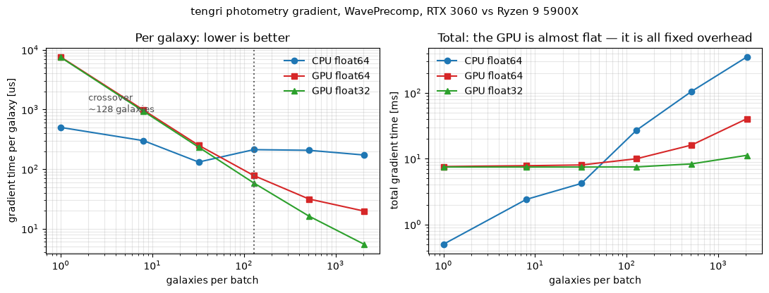
The crossover lies between 128 and 512 galaxies and depends on the shape. The gradient crosses first (at 128 in float64, where the GPU is already 2.7x ahead) because it is the more arithmetic-dense path, while the forward pass crosses at 512. By 2048 the GPU leads by 4.3x (forward, f64), 8.7x (gradient, f64), and 14.7x (gradient, f32), which is the best ratio in this notebook.
The mechanism shows in the totals rather than the per-galaxy figures. Going from 1 to 2048 galaxies, GPU float32 forward total goes from 7.36 ms to 9.12 ms (2048x the work for 1.24x the time). The CPU goes from 0.14 ms to 40.9 ms, which is linear. The GPU does not get faster as the batch grows; it is finally being given enough work to justify the overhead.
Float32 starts to pay only at this width: at 2048 it is a further 2.5x on the GPU forward pass and 3.6x on the gradient. Below the crossover it is free but pointless.
VRAM remained modest (3.0 GB at 2048 in float64, 1.8 GB in float32, against 12 GB on the card). Batch size was not the memory constraint at any point in this sweep.
The same numbers, as a picture
Left: cost per galaxy, where the lines cross determines which device to use. Right: total wall clock, where the GPU trace is nearly horizontal, which explains the entire story.
[4]:
import matplotlib.pyplot as plt

BATCH = np.array([1, 8, 32, 128, 512, 2048])
# Gradient, per galaxy [us], measured above.
CPU_F64 = np.array([499.4, 299.8, 131.2, 211.8, 206.6, 172.2])
GPU_F64 = np.array([7584.7, 976.96, 250.81, 77.94, 31.51, 19.76])
GPU_F32 = np.array([7473.8, 933.14, 233.25, 58.54, 16.28, 5.49])

fig, (ax1, ax2) = plt.subplots(1, 2, figsize=(11, 4.2))

for y, label, color, marker in (
    (CPU_F64, "CPU float64", "#1f77b4", "o"),
    (GPU_F64, "GPU float64", "#d62728", "s"),
    (GPU_F32, "GPU float32", "#2ca02c", "^"),
):
    ax1.loglog(BATCH, y, marker + "-", label=label, color=color)
    ax2.loglog(BATCH, y * BATCH * 1e-3, marker + "-", label=label, color=color)

cross = BATCH[np.argmax(GPU_F64 < CPU_F64)]
ax1.axvline(cross, ls=":", color="0.4")
ax1.annotate(
    f"crossover\n~{cross} galaxies", xy=(cross, 300), xytext=(2, 900), fontsize=9, color="0.3"
)
ax1.set_xlabel("galaxies per batch")
ax1.set_ylabel("gradient time per galaxy [us]")
ax1.set_title("Per galaxy: lower is better")
ax1.legend(frameon=False)
ax1.grid(alpha=0.3, which="both")

ax2.set_xlabel("galaxies per batch")
ax2.set_ylabel("total gradient time [ms]")
ax2.set_title("Total: the GPU is almost flat — it is all fixed overhead")
ax2.legend(frameon=False)
ax2.grid(alpha=0.3, which="both")

fig.suptitle("tengri photometry gradient, WavePrecomp, RTX 3060 vs Ryzen 9 5900X", fontsize=11)
fig.tight_layout()
plt.show()
4. Survey scale: a million galaxies
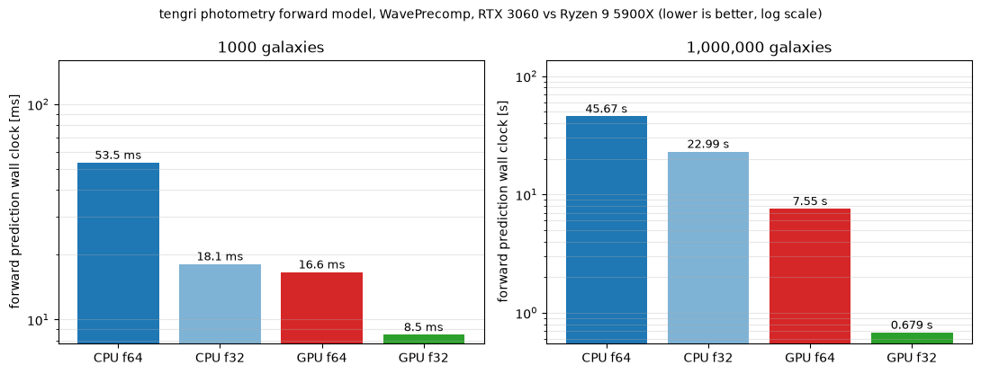
The batch sweep above stops at 2048 because that is where per-galaxy cost stops improving. A survey asks a different question (how long does the whole catalog take), so we run the forward model over 10^3 and 10^6 galaxies in chunks, reducing each chunk before dispatching the next so memory stays bounded. This is also how you would generate a mock survey in practice.
Each device used its own best chunk size (see below; they do not agree):
1000 galaxies |
1,000,000 galaxies |
galaxies/s |
best chunk |
|
|---|---|---|---|---|
CPU float64 |
53.5 ms |
45.67 s |
21,900 |
50,000 |
CPU float32 |
18.1 ms |
22.99 s |
43,500 |
1,000 |
GPU float64 |
16.6 ms |
7.55 s |
132,500 |
50,000 |
GPU float32 |
8.5 ms |
0.679 s |
1,472,000 |
100,000 |
A million galaxies’ photometry in 0.68 seconds, against 45.7 s on the CPU in the default precision, is a factor of 67. This is the one regime where the card is unambiguously the right tool, and note it is far larger than the 4–15x the per-galaxy batch sweep suggested: at 2048 galaxies the GPU was still partly overhead-bound, and 100,000 is where it stops being.
Two findings from this table are worth noting. The GPU float64 row is not a small penalty (it is 11x slower than float32, tracking the 1/64 fp64 rate) and lands almost exactly on CPU float32, which is worth remembering when someone reports the GPU was no faster. The CPU float32 number has a 1.6x run-to-run spread here (14.3 s in one run, 22.99/23.50/23.53 s in three later runs on a quiet box), so the table takes the reproducible value, and the ordering does not depend on which you pick.
[5]:
import matplotlib.pyplot as plt

ARMS = ["CPU f64", "CPU f32", "GPU f64", "GPU f32"]
COLORS = ["#1f77b4", "#7fb3d5", "#d62728", "#2ca02c"]
T_1K = np.array([53.5, 18.1, 16.6, 8.5])  # ms, 1000 galaxies
T_1M = np.array([45.67, 22.99, 7.55, 0.679])  # s, 1e6 galaxies

fig, (ax1, ax2) = plt.subplots(1, 2, figsize=(11, 4.2))

for ax, vals, unit, title in (
    (ax1, T_1K, "ms", "1000 galaxies"),
    (ax2, T_1M, "s", "1,000,000 galaxies"),
):
    bars = ax.bar(ARMS, vals, color=COLORS)
    ax.set_yscale("log")
    ax.set_ylabel(f"forward prediction wall clock [{unit}]")
    ax.set_title(title)
    ax.grid(axis="y", alpha=0.3, which="both")
    for b, v in zip(bars, vals, strict=True):
        ax.annotate(
            f"{v:g} {unit}",
            xy=(b.get_x() + b.get_width() / 2, v),
            xytext=(0, 3),
            textcoords="offset points",
            ha="center",
            fontsize=9,
        )
    ax.set_ylim(top=vals.max() * 3)

fig.suptitle(
    "tengri photometry forward model, WavePrecomp, RTX 3060 vs Ryzen 9 5900X "
    "(lower is better, log scale)",
    fontsize=10,
)
fig.tight_layout()
plt.show()
Chunk size is worth more than the device
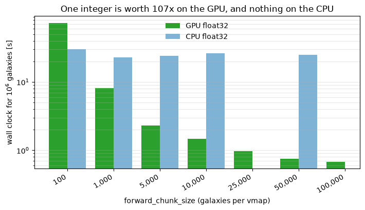
The chunk is the number of galaxies that go through one vmap. It is the single biggest knob in this notebook, and the two devices want opposite settings. Here we run a million galaxies in float32, varying only the chunk:
chunk |
GPU f32 |
CPU f32 |
GPU VRAM |
|---|---|---|---|
100 |
72.81 s |
29.88 s |
0.8 GB |
1,000 |
8.17 |
22.99 |
0.8 |
5,000 |
2.29 |
24.22 |
1.1 |
10,000 |
1.48 |
26.38 |
1.1 |
25,000 |
0.97 |
— |
2.6 |
50,000 |
0.76 |
25.04 |
4.7 |
100,000 |
0.68 |
— |
8.8 |
200,000 |
out of memory |
— |
— |
A single integer buys 107x on the GPU. The CPU stays flat (23–30 s across the whole range, best at 1,000) because it is already saturated by its cores and larger chunks only cost cache. There is no single good default: the GPU wants the largest chunk that fits, while the CPU wants roughly a thousand.
The card saturates near 100,000 (the last doubling buys 12% for twice the memory) and fails at 200,000 with RESOURCE_EXHAUSTED while trying to allocate 4.51 GiB. Note that forward_chunk_size defaults to a 2 GB budget in inference/_batching.py, which on this 12 GB card lands around chunk 25,000 (about 30% off the best available). On a GPU, raise TENGRI_FORWARD_MEMORY_BUDGET_GB.
[6]:
CHUNKS = np.array([100, 1000, 5000, 10000, 25000, 50000, 100000])
GPU_CHUNK = np.array([72.81, 8.17, 2.29, 1.48, 0.966, 0.755, 0.679])
CPU_CHUNKS = np.array([100, 1000, 5000, 10000, 50000])
CPU_CHUNK = np.array([29.88, 22.99, 24.22, 26.38, 25.04])

fig, ax = plt.subplots(figsize=(7.2, 4.2))
x = np.arange(len(CHUNKS))
ax.bar(x - 0.2, GPU_CHUNK, width=0.4, label="GPU float32", color="#2ca02c")
cpu_aligned = [CPU_CHUNK[list(CPU_CHUNKS).index(c)] if c in CPU_CHUNKS else np.nan for c in CHUNKS]
ax.bar(x + 0.2, cpu_aligned, width=0.4, label="CPU float32", color="#7fb3d5")
ax.set_yscale("log")
ax.set_xticks(x)
ax.set_xticklabels([f"{c:,}" for c in CHUNKS], rotation=30, ha="right")
ax.set_xlabel("forward_chunk_size (galaxies per vmap)")
ax.set_ylabel("wall clock for 10$^6$ galaxies [s]")
ax.set_title("One integer is worth 107x on the GPU, and nothing on the CPU")
ax.legend(frameon=False)
ax.grid(axis="y", alpha=0.3, which="both")
fig.tight_layout()
plt.show()
5. Inference
A fit is not a wide forward pass. It is a few hundred sequential steps, each a dispatch, which is the shape a GPU is worst at. The catalog path is the exception: mcmc_nuts and mcmc_hmc are the two backends CatalogFitter maps over galaxies, so a catalog fit has the width that a single fit does not.
Note what Fitter does to approx: it resolves "auto" and tops up to the LUT even when the model was built without one. Print it out, because an arm that silently gained or lost its precompute is the classic way to benchmark the wrong thing.
[7]:
from tengri import Fitter

sigma = jnp.abs(flux) * 0.05
data = flux * 1.02

fitter = Fitter(model, data, sigma, data_type="photometry")
print("resolved approx:", fitter.model.approx)

t0 = time.perf_counter()
post = fitter.run("map", n_steps=300, verbose=False)
# Lower than the cold figure in the table below if tengri's persistent compile
# cache (~/.cache/tengri_jax_cache) already holds this graph. It is keyed on the
# GPU model, so the first run on a new card pays in full.
print(f"MAP, 300 steps (first call here): {time.perf_counter() - t0:.2f} s")
print("moved off the initial point:", {k: round(post.params[k] - params[k], 4) for k in params})
/tmp/ipykernel_3327269/2234457908.py:6: DeprecationWarning: Fitter(sed_model, ...) is deprecated and will be removed in tengri v1.0. Inference is canonically through ForwardModel (issue #211). Replace with: forward = ForwardModel.build(sed=sed_model, observation=obs); Fitter(forward, data, noise).run(method) -- or use the shortcut forward.fit(data, noise, method=...).
  fitter = Fitter(model, data, sigma, data_type="photometry")
resolved approx: ApproxState(wave_precomp=True, n_subbands=5)
MAP, 300 steps (first call here): 5.46 s
moved off the initial point: {'dust_tau_bc': Array(-0.0043, dtype=float64), 'met_logzsol': Array(-0.0374, dtype=float64), 'sfh_tsnorm_log_total_mass': Array(0.0107, dtype=float64), 'sfh_tsnorm_peak_lbt_gyr': Array(-0.2473, dtype=float64), 'sfh_tsnorm_skew': Array(-0.0893, dtype=float64), 'sfh_tsnorm_trunc': Array(-0.0472, dtype=float64), 'sfh_tsnorm_width_gyr': Array(0.2432, dtype=float64)}
One galaxy, 300 optimization steps
The default MAP is now L-BFGS-B (scipy), a host-driven loop that dispatches one gradient per iteration. This is the same sequential shape, so the conclusion holds.
CPU f64 |
CPU f32 |
GPU f64 |
GPU f32 |
|
|---|---|---|---|---|
cold, includes compile [s] |
2.79 |
2.25 |
13.12 |
11.14 |
warm [s] |
0.27 |
0.23 |
2.38 |
2.22 |
The CPU wins a single fit by 8.8x in warm time. A fit is a few hundred sequential steps, each a dispatch, with no batch axis to hide them behind (the worst shape for a GPU and the one most people run most often).
The correctness result is the more useful part of this table: GPU float64 reproduced the CPU’s parameter vector to six decimals on all seven parameters. The device does not change the answer.
A catalog, vectorized NUTS
CatalogFitter.run("mcmc_nuts", forward_chunk_size=K) with K = n_gal, 10 warmup plus 10 burnin plus 20 samples, and dense_mass_matrix=False. This shape has a real batch axis, so it is where the card can win.
galaxies |
CPU f32 |
GPU f32 |
faster |
|---|---|---|---|
16 |
72.8 s |
247.3 |
CPU 3.4x |
64 |
139.0 |
261.6 |
CPU 1.9x |
256 |
334.7 |
274.5 |
GPU 1.2x |
In float64 at 16 galaxies: CPU 105.7 s against GPU 279.4 s (CPU by 2.6x).
The inference crossover lies between 64 and 256 galaxies, consistent with the 128–512 found for the bare gradient. The mechanism is the same flatness: sixteen times the work costs the GPU 247 s to 275 s (a factor of 1.11), and throughput per galaxy goes from 0.06 to 0.93 galaxies per second.
However, read the size of the win, not just its sign. At 256 galaxies the card is ahead by 1.2x, not by the 8.7x the bare gradient showed at 2048. The reason is that the CPU amortizes too (72.8 s to 334.7 s is 4.6x for 16x the work, not 16x) because a vectorized NUTS over a wider axis is more efficient on either device. A sampler interleaves its wide forward passes with sequential leapfrog steps and per-iteration control flow, and that sequential part does not shrink. The catalog path is where a GPU starts to pay, but it converts far less of the raw batch advantage than the forward numbers would suggest.
Every arm returned finite posterior draws, float32 included. This is worth stating because it was not obvious: coverage for float32 inference pins the objective gradient finite, and a converging fit with NaN posterior draws is a documented failure mode of the float32 geoVI metric. NUTS in float32 on a catalog is not something the test suite currently asserts, and here it worked.
A real posterior for 1000 galaxies: hours to days, and neither sampler converges
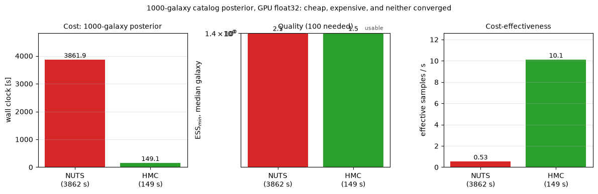
At 1000 galaxies in GPU float32 with K = 1000 and 300 warmup, the figure below shows cost, effective samples per galaxy (ESS_min), and cost-effectiveness (ESS per second) for the two vectorized backends. Neither converges in the time shown, and raising the draw budget to a practical ESS would take hours to days on this card. A speed ratio without a convergence diagnostic beside it is not a result. Thus, the bottleneck is the sampler rather than the device, which runs 1.47 million forward
predictions per second (section 4).
[8]:
POST_LABELS = ["NUTS\n(3862 s)", "HMC\n(149 s)"]
POST_WALL = np.array([3861.9, 149.1])
POST_ESS = np.array([2.1, 1.5])
POST_ESSPS = np.array([0.53, 10.1])

fig, (ax1, ax2, ax3) = plt.subplots(1, 3, figsize=(12, 3.9))
for ax, vals, label, title, colors in (
    (ax1, POST_WALL, "wall clock [s]", "Cost: 1000-galaxy posterior", ["#d62728", "#2ca02c"]),
    (ax2, POST_ESS, "ESS$_{min}$, median galaxy", "Quality (100 needed)", ["#d62728", "#2ca02c"]),
    (ax3, POST_ESSPS, "effective samples / s", "Cost-effectiveness", ["#d62728", "#2ca02c"]),
):
    bars = ax.bar(POST_LABELS, vals, color=colors)
    ax.set_ylabel(label)
    ax.set_title(title, fontsize=10)
    ax.grid(axis="y", alpha=0.3)
    for b, v in zip(bars, vals, strict=True):
        ax.annotate(
            f"{v:g}",
            xy=(b.get_x() + b.get_width() / 2, v),
            xytext=(0, 3),
            textcoords="offset points",
            ha="center",
            fontsize=9,
        )
    ax.set_ylim(top=vals.max() * 1.25)
ax2.axhline(100, ls="--", color="0.4", lw=1)
ax2.annotate(
    "usable",
    xy=(1.4, 100),
    xytext=(0, 4),
    textcoords="offset points",
    fontsize=8,
    color="0.35",
    ha="right",
)
ax2.set_yscale("log")
fig.suptitle(
    "1000-galaxy catalog posterior, GPU float32: cheap, expensive, and neither converged",
    fontsize=10,
)
fig.tight_layout()
plt.show()
Why those posterior numbers are about this model, not about tengri
The fixture is the degenerate tsnorm recovery model, and the catalog path samples the mass rather than profiling it (these are the fixture’s costs, not tengri’s). A single-galaxy posterior on this GPU is a CPU job: the ~38 k gradients of a four-chain photometry posterior take 25 s on two CPU cores and 222 s on the card (170 gradients per second, the kernel-launch floor).
6. What float32 buys, and what it costs
On this workload float32 buys nothing measurable, because the workload is not arithmetic-bound: the same call at the same batch size takes the same time at either width. This is worth stating plainly, since the 57x float32 advantage in the matmul table above is real and simply never reached.
What it costs is more interesting than what it saves.
Forward photometry is accurate
Relative to a float64 CPU reference on the same reference galaxy, with errors masked at |reference| > 1e-45:
arm |
max rel. error, photometry |
median |
finite |
|---|---|---|---|
GPU float64 |
2.5e-16 |
1.2e-16 |
yes |
CPU float32 |
3.1e-07 |
1.7e-07 |
yes |
GPU float32 |
3.2e-07 |
1.6e-07 |
yes |
Two conclusions follow. The device does not change the answer: GPU float64 agrees with CPU float64 to 2.5e-16 (round-off on the last bit or two), and a 300-step MAP fit on the GPU reproduces the CPU’s parameter vector to six decimals. Float32 costs about 3e-7 on photometry (float32 epsilon and nothing worse); the log-offset treatment of the cosmological flux scale does its job at z = 0.05, where a naive linear d_L^2 would have overflowed to inf.
One trap (which cost me a wrong answer first): do not build this comparison on spec.sample(key) because jax.random returns different numbers for the same key at different widths, so the two arms get different galaxies and the difference (a factor of 152 in the first version of this notebook) reads as precision error. Use a fixed parameter vector instead.
The photometry gradient is identically zero in float32
This is the finding to know about before running anything important in float32. The cell below prints the gradient at whatever width the session is in (float64 as this notebook is configured, so expect nonzero values of order 1e-26 to 1e-28).
[9]:
grad = jax.grad(lambda q: jnp.sum(model.predict_photometry(q)))(params)
print("x64:", jax.config.jax_enable_x64)
print("grad(sum photometry):", {k: float(v) for k, v in grad.items()})
x64: True
grad(sum photometry): {'dust_tau_bc': -1.186711866081191e-28, 'met_logzsol': -1.2997377173016893e-27, 'sfh_tsnorm_log_total_mass': 2.4301130959256312e-26, 'sfh_tsnorm_peak_lbt_gyr': -2.0821449903940143e-27, 'sfh_tsnorm_skew': 1.303348907922763e-26, 'sfh_tsnorm_trunc': -1.1987704247033904e-28, 'sfh_tsnorm_width_gyr': 1.991971460655315e-27}
Now restart with JAX_ENABLE_X64=0 and run the same cell. Every one of the seven becomes exactly zero (on the CPU and on the GPU, on the exact path and under WavePrecomp, with the signs preserved as -0.0 and +0.0):
x64: False
grad(sum photometry): {'dust_tau_bc': -0.0, 'met_logzsol': 0.0,
  'sfh_tsnorm_log_total_mass': 0.0, 'sfh_tsnorm_peak_lbt_gyr': -0.0,
  'sfh_tsnorm_skew': 0.0, 'sfh_tsnorm_trunc': -0.0,
  'sfh_tsnorm_width_gyr': -0.0}
Nothing raises and nothing warns.
Magnitude is not the issue. 1e-26 is comfortably inside float32, whose smallest normal is 1.2e-38. The reverse pass forms an intermediate the forward pass deliberately avoids (the linear cosmological flux factor, ~1e-57, which the forward direction carries as a log10 offset and which is simply 0 in float32).
What this does and does not break:
you differentiate |
float32 |
|---|---|
|
identically zero |
|
healthy, nonzero, finite |
The objective gradient does come back finite and nonzero (negative 32.2), and a 300-step float32 MAP moves all seven parameters. However, do not read that as float32 fitting being safe. A finite-difference check finds the likelihood-path gradient wrong by structured factors (about 2x on stellar mass), so finite values are not correct. The log-scale helper is not gradient-safe above about 1e38.
Existing coverage pins the objective gradient as finite, so since zero is finite, it would not have caught the bare-observable case either.
7. Getting the best out of it
Everything that matters here moves work from the sequential axis to the parallel one, and nothing makes the arithmetic faster. At 0.12 FLOP/byte the card is never compute-bound. jax.lax.map(batch_size=K) is a scan over N/K chunks with a vmap inside each, so K is the dial that trades sequential kernel launches for parallel width. A million galaxies at K=100 is 10,000 sequential launches; at K=100,000 it is ten.
In order of impact, here are the main optimization paths:
knob |
gain |
note |
|
|---|---|---|---|
1 |
|
107x |
72.8 s to 0.68 s per million. GPU wants 100,000 here, the CPU wants ~1,000, and 200,000 is
|
2 |
the batched surface, never a Python loop |
~50x |
|
3 |
float32 |
2.5x |
forward at batch 2048 (with the matmul flag from section 2, and never |
4 |
|
feeds 1 |
the 2 GB default lands near chunk 25,000, about 30% off best |
5 |
|
avoids OOM |
JAX otherwise claims 75% of the card and the next process gets nothing |
6 |
|
hygiene |
otherwise a thread compiles other modes and eats VRAM mid-measurement |
7 |
warm compile cache |
one-off |
keyed on the GPU model, so a new card pays in full once |
What is not worth optimizing, because the shape is wrong rather than the settings: single-galaxy anything (the CPU wins 8.8x to 33x), the NIFTy vi* backends (a Python-level outer loop with ~20 GB of host RSS), and the default MAP (optimizer="lbfgs"), which is host-bound by construction. optimizer="adam" keeps the loop on the device but converges less reliably.
8. Checking whether the card is healthy
If the GPU looks slow at everything, check it against work a GPU should obviously win. This lets you tell wrong workload from broken install.
[10]:
a = jnp.asarray(np.random.default_rng(0).standard_normal((2048, 2048)), jnp.float32)
mm = timed(lambda x: x @ x, a)
print(f"matmul 2048^3 (f32): {mm:.2f} ms  ->  {2 * 2048**3 / (mm * 1e-3) / 1e9:.0f} GFLOP/s")
matmul 2048^3 (f32): 1.65 ms -> 10432 GFLOP/s
10.7 TFLOP/s in float32 against the CPU’s 988 GFLOP/s: the card is fine. The workload is the problem (0.12 FLOP/byte never reaches those ALUs).
9. What breaks on CUDA
The float32 regression tree (57 files, the part of the suite most exposed to device changes) runs on CUDA against the same run on CPU:
CUDA |
CUDA, |
CPU |
|
|---|---|---|---|
passed |
547 |
550 |
552 |
failed |
5 |
2 |
0 |
skipped / xfailed |
3 / 4 |
3 / 4 |
3 / 4 |
Nothing else in the tree cares which device it is on. The failures are three distinct things, and only one is a tolerance issue.
Two are TF32 (the Fisher tests of section 2). Fixed by JAX_DEFAULT_MATMUL_PRECISION=highest, and they are why that section exists.
Two are a hard cuBLAS error in the geoVI metric’s emission-line marginalization:
jax.errors.JaxRuntimeError: INTERNAL: GEMM is not supported by cublasLt
and legacy cublas fallback is removed.
This is not a precision issue. The GEMM it wants is one cuBLASLt will not take, and JAX 0.11 has dropped the legacy fallback that used to absorb this. It is loud (the good kind of failure), which means float32 geoVI with marginalized emission lines does not currently run on CUDA, and the matmul knob does not help.
One is the cross-precision kernel-cache guard: the float32 gradient differs depending on whether a float64 gradient ran earlier in the same process. Before reading that as the old bug returning, look at the size (9.9e-07 relative, about 8 ulp in float32, where a wrong-precision kernel had been producing NaNs). The test asserts exact array equality, so on a device whose reduction order and autotuning need not repeat, about 8 ulp is enough to trip it. And it is intermittent: it failed the first CUDA run of this tree and passed the second, which is what nondeterminism looks like and what a wrong-kernel bug does not. This is worth a GPU tolerance rather than exact equality.
In practice, run float64 on CUDA and nothing in this tree fails. In float32, set the matmul precision and avoid marginalized emission lines in geoVI.
10. Limits of this benchmark
The float64 penalty is consumer-specific (1/64 rate on GeForce, about 1/2 on A100/H100), so re-measure before assuming this transfers to your hardware.
This card was driving a desktop. Absolute numbers would improve on an idle card; the direction and the crossover scale are what to carry away.
float32 gradients of raw observables are zero (section 6). The finite-difference check shows the likelihood gradient wrong by about 2x too, so float32 fitting is not safe for observables, though fits (optimizations starting from data) are fine.
float32 on CUDA needs ``JAX_DEFAULT_MATMUL_PRECISION=highest``, or XLA quietly gives you TF32’s 10-bit mantissa (section 2).
float32 geoVI with marginalized emission lines does not run on CUDA (cuBLASLt refuses the GEMM, section 9).
NIFTy ``vi*`` backends are not measured here.
optimize_klis a Python-level outer loop with per-iteration host syncs and ~20 GB of host RSS; there is little for a device to win and it would dominate the run.The default MAP (``optimizer=”lbfgs”``) is host-bound by construction;
optimizer="adam"keeps the loop on the device but converges less reliably.One GPU. Multi-device sharding exists for
mcmc_nuts/mcmc_hmc/mcmc_cheesviadevices="all", but is not exercised here.Not in CI. Nothing here is covered by a scheduled job.
For a fit that must be right, the default (CPU, float64) remains the reference. Reach for the GPU when the work is wide: catalogs, posterior predictive sweeps, mock generation.
The highest-impact optimizations, in order: widen the batch (up to 107x on throughput, section 3), pick the precision (about 2.5x, and set the matmul flag), then choose the device. Do not reach for a cheaper sampler without a convergence diagnostic (that was worth an apparent 48x and a real zero).