Which parts of a bursty star-formation history can you actually measure?
⚠️ Experimental. A research demonstration using experimental APIs that may change between releases.
Star formation is bursty: it flickers on tens-to-hundreds-Myr timescales. Tengri models this directly as a smooth backbone times a stochastic Gaussian-process field governed by a power spectrum:
The problem: the field adds one free parameter per age bin, so it can fit almost any history. A fit will always return bursts, whether the data measured them or not. We ask which parts of the SFH answer are real, and which are the prior.
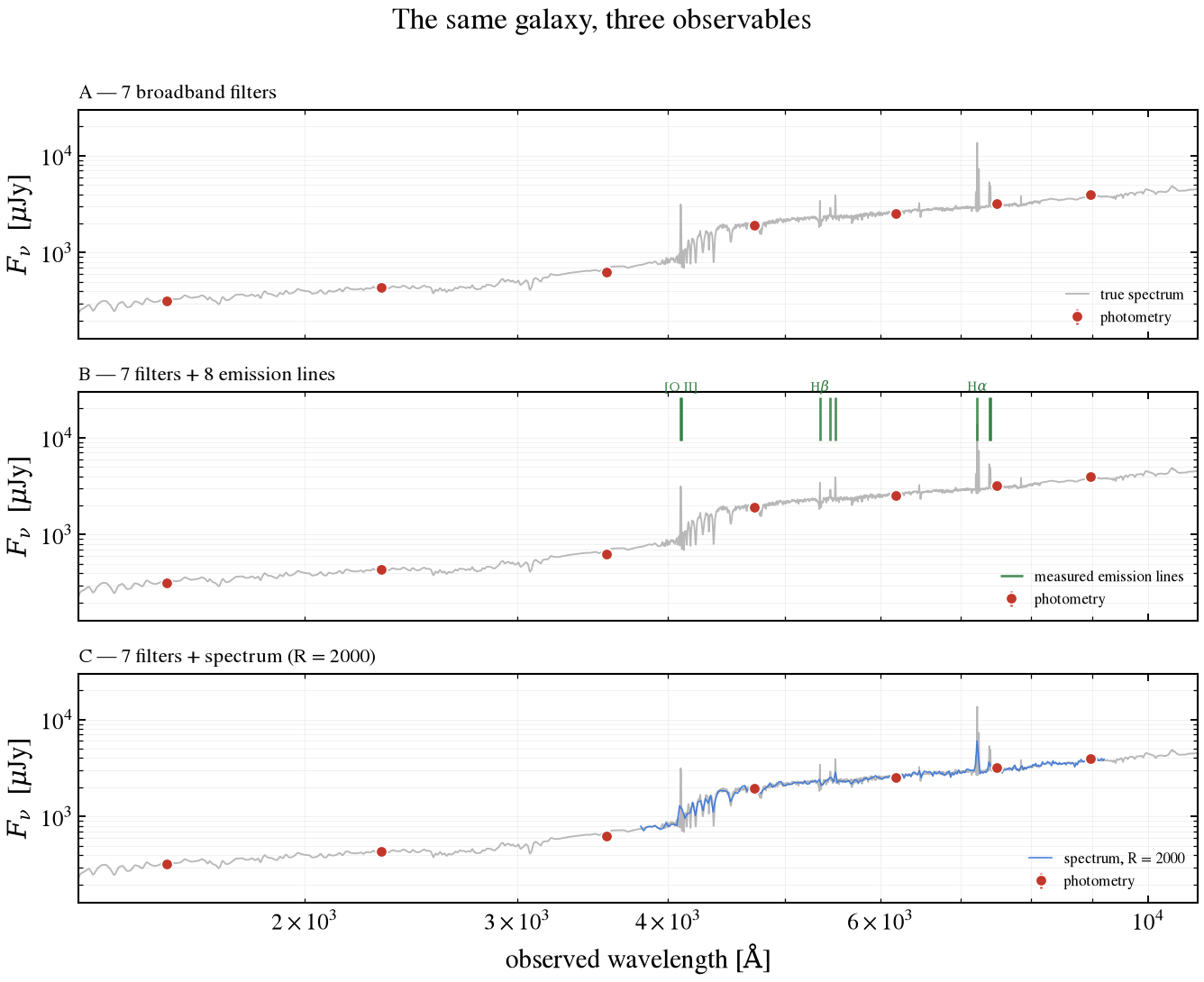
This notebook injects one known bursty history into a galaxy and observes it three ways:
Observable |
Constrains |
|---|---|
7 broadband filters (GALEX → SDSS z) |
overall shape, stellar mass |
Same + 8 optical emission lines |
the last 15 Myr, directly |
Same + R = 2000 optical spectrum |
the above, plus old mass budget |
Truth, model, noise, and random seed stay fixed across all three. Only the observable changes, so any difference in the recovered history reflects the information content of the data.
[1]:
import warnings

# _setup must be imported BEFORE jax: it sets TF_CPP_MIN_LOG_LEVEL, which XLA only
# reads at import. Import jax first and every cell below carries a wall of
# "PjRt-IFRT does not track XLA executable versions" into the rendered page.
#
# FIG_DIR arrives anchored on _setup's own location, so figures land in
# notebooks/_figs wherever this was started from. The SSP goes through
# tengri.load_ssp for the same reason: a working-directory-relative grid path
# misses silently and falls through to a 67 MB download.
from _plot_style import setup_style
from _setup import FIG_DIR, effective_wavelengths_um, quiet

quiet()
setup_style()

# Two notices that are correct, and correct to ignore *here*:
#   - a wNE library warns that nebular emission is already in the templates and must
#     be paired with the baked-in backend, which is exactly the pairing used below;
#   - two_component(all_params=FREE) frees the two Calzetti optical depths and reports
#     that Rv, delta, the bump strength and the obscured fraction stay fixed. They
#     belong to other attenuation laws, and holding them constant is the point: this
#     notebook varies the star-formation history, not the dust law.
warnings.filterwarnings("ignore", message=r"(?s).*is a wNE .*")
warnings.filterwarnings("ignore", message=r"(?s).*run with that physics held constant.*")

import time

import jax
import jax.numpy as jnp

jax.config.update("jax_enable_x64", True)

import matplotlib.pyplot as plt
import numpy as np

import tengri
from tengri import (
    builders,
    DEFAULT,
    Fixed,
    ForwardModel,
    FREE,
    NoiseModel,
    Observation,
    Photometry,
    SEDModel,
    Spectroscopy,
    WavePrecomp,
)
from tengri.observation import LineFluxData
from tengri.observation.line_measurement import default_line_defs
from tengri.plot import plot_sfh

# One color per observable, used consistently in every figure below.
C = {"A": "#8c8c8c", "B": "#2f7d3f", "C": "#3a76d9"}
C_TRUTH = "0.05"
1. The galaxy, and the three ways we observe it
A wNE stellar library bakes nebular emission into the templates, so the Balmer and forbidden lines that trace the last few megayears come along with the stellar continuum. No separate emission model is needed, and the line fluxes are measured off the model spectrum the way a pipeline measures data.
[2]:
SSP_NAME = "ssp_prsc_miles_chabrier_wNE_logGasU-3.0_logGasZ0.0"
ssp_data = tengri.load_ssp(SSP_NAME)

# An SDSS-like galaxy: GALEX ultraviolet (which is where dust bites) through the
# SDSS optical.
BANDS = ["galex_fuv", "galex_nuv", "sdss_u", "sdss_g", "sdss_r", "sdss_i", "sdss_z"]

# Strong star-forming optical lines. Hgamma and [NII] are left out on purpose:
# they sit on top of stellar Balmer absorption and measure near zero for these
# histories, so their signal-to-noise-scaled errors would feed the fit pure noise.
LINE_NAMES = [
    "Halpha",
    "Hbeta",
    "OIII_5007",
    "OIII_4959",
    "SII_6717",
    "SII_6731",
    "OII_3726",
    "OII_3729",
]

WAVE_OBS = jnp.linspace(3800.0, 9200.0, 260)  # rest 3455-8364 A at z = 0.1

Z_GAL = 0.1
N_GRID = 16  # field latents; Section 1 prints the total dimension they add up to
PHOT_SNR, LINE_SNR, SPEC_SNR = 20.0, 10.0, 30.0

phot = Photometry.from_names(BANDS)
noise_model = NoiseModel(calibration_floor=0.01, student_t_dof=None)

# A template LineFluxData fixes *which* lines the model is built to fit; the
# observed values are filled in per galaxy below.
line_template = LineFluxData.from_dict({nm: (1e-16, 1e-17) for nm in LINE_NAMES})
line_defs = default_line_defs(np.asarray(line_template.wavelengths), tuple(line_template.names))
spec_obs = Spectroscopy(WAVE_OBS, resolution=2000)

# The three observables. Same filters throughout; each adds one thing.
OBSERVATION = {
    "A": Observation(photometry=phot, noise=noise_model),
    "B": Observation(photometry=phot, line_fluxes=line_template, noise=noise_model),
    "C": Observation(photometry=phot, spectroscopy=spec_obs, noise=noise_model),
}
LABEL = {
    "A": f"{len(BANDS)} broadband filters",
    "B": f"{len(BANDS)} filters + {len(LINE_NAMES)} emission lines",
    "C": f"{len(BANDS)} filters + spectrum (R = 2000)",
}


#: The SSP x filter lookup table shared by every fit on this page. One instance
#: across all three observables (see the note under the builds below).
FAST_PATH = WavePrecomp()


def build(observation, n_grid=N_GRID, approx=FAST_PATH):
    """The same physical model behind all three fits, on one observable.

    A rising double power law (Carnall et al. 2018) — a galaxy still forming stars,
    not a quiescent one — modulated by the stochastic field. Dust is two-component
    Calzetti with both optical depths free; metallicity and redshift are fixed so
    the comparison isolates the star-formation history.
    """
    return SEDModel.build(
        ssp_data=ssp_data,
        observation=observation,
        sfh={"type": ["dpl", "field"], "all_params": FREE},
        met={"logzsol": Fixed(-0.3), "all_params": Fixed(DEFAULT)},
        dust_attenuation=builders.dust.two_component(all_params=FREE, law="calzetti"),
        neb=builders.neb.ssp(),
        redshift=Fixed(Z_GAL),
        igm={"type": "none"},
        n_grid=n_grid,
        approx=approx,
    )


# Every model here rides the `WavePrecomp` SSP x filter table (the `build` default
# above). The lookup table cuts one forward pass from 6.66 ms to 0.10 ms. The
# posterior below gains only about 1.5× because most of its cost is the field prior
# and the dense metric. The table takes about a second to build.
model = {k: build(v) for k, v in OBSERVATION.items()}
spec = model["B"].spec
print(
    f"SFH dimension: {spec.n_grid} field latents + {spec.n_free} physical "
    f"= D {spec.n_grid + spec.n_free}"
)
SFH dimension: 16 field latents + 9 physical = D 25
src/tengri/forward/sed_model.py:3690: UserWarning: 132/260 (50.8%) spectral pixels have instrument resolution narrower than SSP library 'ssp_prsc_miles_chabrier_wNE_logGasU-3.0_logGasZ0.0''s own LSF at z=0.1: sigma_inst^2 - sigma_lib^2 is clamped to zero there (no broadening applied) rather than raising, which under-broadens the model in that unresolvable regime (#2518). (50 of those also fall in the library's approximate, FSPS-extrapolated resolution range rather than its own measured templates.) Use a coarser instrument resolution or a library with finer native resolution at these wavelengths.
  self._init_instrument(spec, observation)
2. One known history, injected
The truth is a rising backbone with a moderately bursty field on top (\(\sigma = 0.4\) dex, \(\tau = 120\) Myr, the molecular-cloud decorrelation time of Tacchella, Forbes & Caplar 2020). We rescale the mass so the mean present-day rate is 20 \(M_\odot\) yr\(^{-1}\), which leaves the rising shape and the bursts untouched.
[3]:
SEED = 1
DPL = {
    "sfh_dpl_alpha": 2.0,
    "sfh_dpl_beta": 1.5,
    "sfh_dpl_age_frac": 12.0 / tengri.utils.cosmology.age_at_z(Z_GAL),  # 12 Gyr at z = 0.1
    "sfh_dpl_tau_gyr": 13.0,
}

truth = {
    **spec.sample(jax.random.PRNGKey(SEED)),  # a field realization, xi ~ N(0, I)
    **{k: jnp.array(v) for k, v in DPL.items()},
    "dust_tau_bc": jnp.array(0.3),
    "dust_tau_diff": jnp.array(0.15),
    "sfh_field_psd_sigma": jnp.array(0.4),
    "sfh_field_psd_tau_myr": jnp.array(120.0),
    "sfh_dpl_log_total_mass": jnp.array(11.0),
}
_sfh = model["B"].predict_sfh(truth)
_now = int(np.argmin(np.asarray(_sfh["t_gyr"])))  # present = smallest lookback time
truth["sfh_dpl_log_total_mass"] = jnp.array(
    11.0 + np.log10(20.0 / float(np.asarray(_sfh["sfr_mean"])[_now]))
)
# Score on the model's OWN log-age nodes, not the default linear resampling: the
# linear grid steps by age_max / n_linear = 13.8 Myr, so only 2 of its samples fall
# below 15 Myr while 5 of the 16 log-age nodes do. Scoring on the linear grid
# weights every megayear equally and lets 15-500 Myr swamp the young bins.
nodes = model["B"].predict_sfh(truth, grid="native")
t_node = np.asarray(nodes["t_gyr"])
sfr_true = np.asarray(nodes["sfr_full"])

YOUNG_GYR, MID_GYR = 0.015, 1.0
WINDOW = {
    "recent (< 15 Myr)": t_node < YOUNG_GYR,
    "intermediate (15 Myr - 1 Gyr)": (t_node >= YOUNG_GYR) & (t_node < MID_GYR),
    "old (> 1 Gyr)": t_node >= MID_GYR,
}
print(
    f"Injected SFH on {t_node.size} log-age nodes, "
    f"{t_node.min() * 1e3:.1f} Myr to {t_node.max():.1f} Gyr"
)
Injected SFH on 16 log-age nodes, 1.0 Myr to 12.4 Gyr
Synthesizing the three data sets
All three observables are drawn from the same truth at S/N 20 (photometry), 10 (lines), 30 (spectrum).
[4]:
mock = model["A"].mock(
    truth,
    snr=PHOT_SNR,
    key=jax.random.PRNGKey(SEED + 10_000),
)
flux_phot, err_phot = np.asarray(mock.flux_obs), np.asarray(mock.noise)

# measure_line_fluxes needs its line_defs passed explicitly. Left out, it falls
# back to a built-in DESI set of five lines -- not the eight this Observation
# declares -- and the returned array would silently describe different lines.
lf_true = np.asarray(model["B"].measure_line_fluxes(truth, line_defs))
assert lf_true[LINE_NAMES.index("Halpha")] > 0, "Halpha not in emission for this truth"
err_line = np.abs(lf_true) / LINE_SNR
flux_line = lf_true + err_line * np.random.default_rng(SEED + 20_000).standard_normal(
    lf_true.shape
)

spec_true = np.asarray(model["C"].predict_spectrum(truth, wave_obs=WAVE_OBS))
err_spec = np.abs(spec_true) / SPEC_SNR
flux_spec = spec_true + err_spec * np.random.default_rng(SEED + 30_000).normal(
    size=spec_true.shape
)

# Fold the measured values into the observations the fits will actually see.
line_data = LineFluxData(
    names=tuple(LINE_NAMES),
    fluxes=jnp.asarray(flux_line),
    errors=jnp.asarray(err_line),
    wavelengths=line_template.wavelengths,
)
OBSERVATION["B"] = Observation(photometry=phot, line_fluxes=line_data, noise=noise_model)

DATA = {
    "A": (flux_phot, err_phot),
    "B": (flux_phot, err_phot),
    # Photometry and spectrum arrive as one concatenated vector; the Observation
    # already declares both, so the split is unambiguous.
    "C": (np.concatenate([flux_phot, flux_spec]), np.concatenate([err_phot, err_spec])),
}
print(
    f"A: {flux_phot.size} fluxes   "
    f"B: {flux_phot.size} + {flux_line.size} lines   "
    f"C: {flux_phot.size} + {flux_spec.size} spectral pixels"
)
A: 7 fluxes B: 7 + 8 lines C: 7 + 260 spectral pixels
What each observable sees
The faint gray curve is the same true spectrum in all three panels; the markers differ.
[5]:
wave_wide = jnp.linspace(1300.0, 11000.0, 3000)
sed_wide = np.asarray(model["C"].predict_spectrum(truth, wave_obs=wave_wide))
TO_UJY = 1e29  # erg/s/cm2/Hz -> microjansky
wave_eff = np.asarray(effective_wavelengths_um(phot)) * 1e4

X_LO, X_HI = 1300.0, 11000.0
# Set the limits from the noiseless SED, not from the data. The noisy spectrum has
# pixels scattered close to zero, and on a shared log axis those would drag the
# lower limit down two decades and leave every panel mostly empty.
_shown = (np.asarray(wave_wide) >= X_LO) & (np.asarray(wave_wide) <= X_HI)
Y_LO = float(np.nanmin(sed_wide[_shown])) * TO_UJY * 0.55
Y_HI = float(np.nanmax(sed_wide[_shown])) * TO_UJY * 2.2

# Three well-separated lines to name. [O III] 5007 is deliberately left unlabeled:
# at this width its tick sits ~160 A from Hbeta and the two labels overlap into
# nonsense. All eight are still drawn.
NAMED = {"OII_3726": "[O II]", "Hbeta": r"H$\beta$", "Halpha": r"H$\alpha$"}

fig, axes = plt.subplots(3, 1, figsize=(9.2, 7.4), sharex=True, sharey=True)
for key, ax in zip("ABC", axes):
    ax.plot(
        np.asarray(wave_wide),
        sed_wide * TO_UJY,
        color="0.72",
        lw=0.9,
        zorder=1,
        label="true spectrum" if key == "A" else None,
    )
    if key == "C":
        ax.plot(
            np.asarray(WAVE_OBS),
            flux_spec * TO_UJY,
            color=C["C"],
            lw=0.8,
            alpha=0.9,
            zorder=2,
            label="spectrum, R = 2000",
        )
    if key == "B":
        obs_wl = np.asarray(line_template.wavelengths) * (1 + Z_GAL)
        ax.vlines(
            obs_wl,
            Y_HI / 3.2,
            Y_HI / 1.15,
            color=C["B"],
            lw=1.3,
            alpha=0.85,
            zorder=3,
            label="measured emission lines",
        )
        for nm, tex in NAMED.items():
            ax.text(
                obs_wl[LINE_NAMES.index(nm)],
                Y_HI / 1.08,
                tex,
                color=C["B"],
                fontsize=7.5,
                ha="center",
                va="bottom",
            )
    ax.errorbar(
        wave_eff,
        flux_phot * TO_UJY,
        yerr=err_phot * TO_UJY,
        fmt="o",
        ms=6,
        color="#c3372a",
        mec="w",
        mew=0.8,
        lw=1.2,
        zorder=4,
        label="photometry",
    )
    ax.set_xscale("log")
    ax.set_yscale("log")
    ax.set_ylabel(r"$F_\nu$  [$\mu$Jy]")
    ax.set_title(f"{key} — {LABEL[key]}", loc="left", fontsize=10.5)
    ax.legend(fontsize=8, loc="lower right", framealpha=0.92)
    ax.grid(alpha=0.2, which="both", lw=0.4)
axes[-1].set_xlabel(r"observed wavelength [$\mathrm{\AA}$]")
axes[-1].set_xlim(X_LO, X_HI)
axes[-1].set_ylim(Y_LO, Y_HI)
fig.suptitle("The same galaxy, three observables", y=0.995)
fig.tight_layout()
fig.savefig(FIG_DIR / "sfh_observables.png", dpi=150, bbox_inches="tight")
plt.show()
3. Fit all three
MAP fits to find the mode of each posterior. A full posterior (Section 5) covers the middle case.
[6]:
fits, timings = {}, {}
for key in "ABC":
    obs = OBSERVATION[key]
    m = build(obs)
    data, err = DATA[key]
    t0 = time.perf_counter()
    fits[key] = ForwardModel.build(sed=m, observation=obs).fit(
        data,
        err,
        method="map",
        n_restarts=3,
        key=jax.random.PRNGKey(SEED),
        verbose=False,
    )
    timings[key] = time.perf_counter() - t0
    model[key] = m
    print(f"{key}: MAP in {timings[key]:5.1f} s")
A: MAP in   7.6 s
B: MAP in  47.0 s
src/tengri/forward/sed_model.py:3690: UserWarning: 132/260 (50.8%) spectral pixels have instrument resolution narrower than SSP library 'ssp_prsc_miles_chabrier_wNE_logGasU-3.0_logGasZ0.0''s own LSF at z=0.1: sigma_inst^2 - sigma_lib^2 is clamped to zero there (no broadening applied) rather than raising, which under-broadens the model in that unresolvable regime (#2518). (50 of those also fall in the library's approximate, FSPS-extrapolated resolution range rather than its own measured templates.) Use a coarser instrument resolution or a library with finer native resolution at these wavelengths.
  self._init_instrument(spec, observation)
C: MAP in 110.5 s
4. What came back
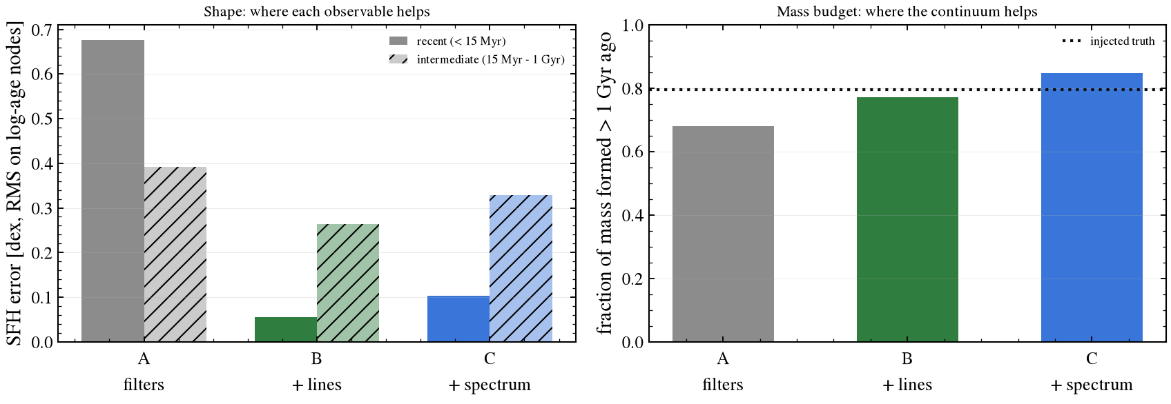
Two scores per fit:
RMS error in dex (per age window): recovery accuracy of the SFH shape.
Old mass fraction: the fraction of stellar mass formed > 1 Gyr ago. Use mass, not per-node SFR, because below 1 Gyr the rising history has near-zero rate where per-node error ratios diverge.
[7]:
def sfr_at_nodes(key):
    """MAP star-formation rate on the native log-age nodes [Msun/yr]."""
    return np.asarray(model[key].predict_sfh(fits[key].params, grid="native")["sfr_full"])


def rms_dex(pred, mask):
    lo = 1e-8
    return float(
        np.sqrt(
            np.mean(
                (
                    np.log10(np.clip(pred[mask], lo, None))
                    - np.log10(np.clip(sfr_true[mask], lo, None))
                )
                ** 2
            )
        )
    )


def old_mass_fraction(sfr):
    """Fraction of stellar mass formed more than 1 Gyr ago."""
    order = np.argsort(t_node)
    t, s = t_node[order], np.asarray(sfr)[order]
    total = np.trapezoid(s, t)
    old = t > MID_GYR
    return float(np.trapezoid(s[old], t[old]) / total) if total > 0 else np.nan


sfr_map = {k: sfr_at_nodes(k) for k in "ABC"}
score = {
    k: {name: rms_dex(sfr_map[k], mask) for name, mask in WINDOW.items()}
    | {"f_old": old_mass_fraction(sfr_map[k])}
    for k in "ABC"
}
f_old_true = old_mass_fraction(sfr_true)

print(f"{'':38s}{'recent':>9s}{'interm.':>9s}{'f_old':>9s}")
print("-" * 65)
for k in "ABC":
    s = score[k]
    print(
        f"{k} {LABEL[k]:36s}"
        f"{s['recent (< 15 Myr)']:>9.3f}"
        f"{s['intermediate (15 Myr - 1 Gyr)']:>9.3f}"
        f"{s['f_old']:>9.3f}"
    )
print(f"{'':38s}{'':>9s}{'':>9s}{f_old_true:>9.3f}  <- truth")
                                         recent  interm.    f_old
-----------------------------------------------------------------
A 7 broadband filters                     0.677    0.392    0.679
B 7 filters + 8 emission lines            0.055    0.264    0.771
C 7 filters + spectrum (R = 2000)         0.103    0.329    0.847
                                                            0.796  <- truth
src/tengri/components/stellar/component.py:765: SFHBeyondSSPGridWarning: The tabulated star formation history forms 1% of its stellar mass at lookback ages older than the oldest SSP template (12.59 Gyr). No template represents stars that old, so that mass is assigned to the oldest one: the total is conserved, but those stars carry the colors of a 12.59 Gyr population rather than their true age. Use an SSP grid that spans the galaxy's age, or start the history later, to remove the approximation.
  _warn_if_history_exceeds_ssp_grid(fine_age_yr, sfr, ssp_ages_yr, tab_lbt_yr)
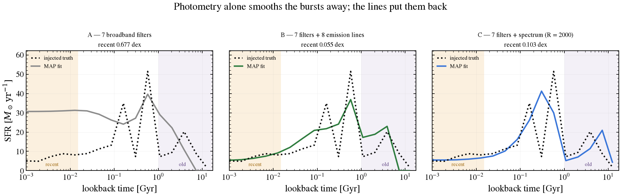
The recovered histories
Linear SFR axis (true for mass budget) on log time axis (to separate recent age bins).
[8]:
fig, axes = plt.subplots(1, 3, figsize=(13.6, 4.3), sharey=True)
top = float(np.nanmax([sfr_true.max()] + [sfr_map[k].max() for k in "ABC"])) * 1.12
t_plot = np.clip(t_node, 1e-3, None)

for key, ax in zip("ABC", axes):
    ax.axvspan(t_plot.min(), YOUNG_GYR, color="#e8a33d", alpha=0.16, lw=0)
    ax.axvspan(MID_GYR, t_plot.max() * 1.4, color="#8f6fb5", alpha=0.10, lw=0)
    ax.plot(t_plot, sfr_true, color=C_TRUTH, lw=2.2, ls=":", label="injected truth", zorder=4)
    ax.plot(t_plot, sfr_map[key], color=C[key], lw=2.2, label="MAP fit", zorder=3)
    ax.set_xscale("log")
    ax.set_xlim(t_plot.min(), t_plot.max() * 1.4)
    ax.set_ylim(0, top * 1.08)
    ax.set_xlabel("lookback time [Gyr]")
    ax.set_title(
        f"{key} — {LABEL[key]}\nrecent {score[key]['recent (< 15 Myr)']:.3f} dex", fontsize=10
    )
    ax.legend(fontsize=8.5, loc="upper left", framealpha=0.92)
    ax.grid(alpha=0.22, lw=0.4)
axes[0].set_ylabel(r"SFR [$M_\odot\,\mathrm{yr}^{-1}$]")
# Window labels sit at the FOOT of each shaded band: at the top they collide with
# the legend, and the SFR curves never come near the floor on the left.
for _ax in axes:
    _ax.text(
        np.sqrt(t_plot.min() * YOUNG_GYR),
        top * 0.03,
        "recent",
        fontsize=8,
        color="#a06a10",
        ha="center",
        va="bottom",
    )
    _ax.text(
        np.sqrt(MID_GYR * t_plot.max()),
        top * 0.03,
        "old",
        fontsize=8,
        color="#5c4080",
        ha="center",
        va="bottom",
    )
fig.suptitle("Photometry alone smooths the bursts away; the lines put them back", y=1.0)
fig.tight_layout()
fig.savefig(FIG_DIR / "sfh_recovery_by_observable.png", dpi=150, bbox_inches="tight")
plt.show()
The scorecard
[9]:
fig, (ax_dex, ax_mass) = plt.subplots(1, 2, figsize=(11.6, 4.2))
x = np.arange(3)
w = 0.36
for i, (name, off) in enumerate(
    (("recent (< 15 Myr)", -w / 2), ("intermediate (15 Myr - 1 Gyr)", +w / 2))
):
    ax_dex.bar(
        x + off,
        [score[k][name] for k in "ABC"],
        w,
        color=[C[k] for k in "ABC"],
        alpha=1.0 if i == 0 else 0.45,
        hatch=None if i == 0 else "//",
        label=name,
    )
ax_dex.set_xticks(x)
ax_dex.set_xticklabels(["A\nfilters", "B\n+ lines", "C\n+ spectrum"])
ax_dex.set_ylabel("SFH error [dex, RMS on log-age nodes]")
ax_dex.set_title("Shape: where each observable helps", fontsize=10.5)
ax_dex.legend(fontsize=8.5)
ax_dex.grid(axis="y", alpha=0.3, lw=0.4)

ax_mass.bar(x, [score[k]["f_old"] for k in "ABC"], 0.55, color=[C[k] for k in "ABC"])
ax_mass.axhline(f_old_true, color=C_TRUTH, ls=":", lw=2.0, label="injected truth")
ax_mass.set_xticks(x)
ax_mass.set_xticklabels(["A\nfilters", "B\n+ lines", "C\n+ spectrum"])
ax_mass.set_ylabel("fraction of mass formed > 1 Gyr ago")
ax_mass.set_ylim(0, 1)
ax_mass.set_title("Mass budget: where the continuum helps", fontsize=10.5)
ax_mass.legend(fontsize=8.5)
ax_mass.grid(axis="y", alpha=0.3, lw=0.4)

fig.tight_layout()
fig.savefig(FIG_DIR / "sfh_scorecard.png", dpi=150, bbox_inches="tight")
plt.show()
5. Full posterior inference
The MAP comparison shows where the mode lands and how wide the posterior is. With 15 measured numbers (7 fluxes, 8 lines) and the model dimension in Section 1, the width matters. We run a Hamiltonian Monte Carlo posterior on case B.
The emission-line channel keeps the stellar mass inside the sampler and the model has 25 free parameters, so a fixed-length HMC trajectory with a dense metric keeps the cost predictable. The posterior is wide and strongly correlated; the non-centered field rotates with \(\tau\), so the curvature is position-dependent. This is a single chain, and its split R-hat printed below stays above the 1.01 convergence bar: read the bands as the shape of the recovered history, not as calibrated credible intervals.
[10]:
# Trajectory length sets the cost; this demonstration budget runs in tens of minutes.
t0 = time.perf_counter()
posterior = ForwardModel.build(sed=model["B"], observation=OBSERVATION["B"]).fit(
    *DATA["B"],
    method="mcmc_hmc",
    init_from=fits["B"],
    n_warmup=1000,
    n_samples=400,
    n_leapfrog_steps=100,
    dense_mass_matrix=True,
    key=jax.random.PRNGKey(SEED + 7),
    verbose=False,
)
print(f"HMC in {time.perf_counter() - t0:.0f} s")
HMC in 1271 s
[11]:
rhat = {k: float(v) for k, v in posterior.rhat().items()}
worst = max(rhat, key=lambda k: rhat[k] if np.isfinite(rhat[k]) else np.inf)
max_rhat = float(np.nanmax(list(rhat.values())))
print(f"max R-hat {max_rhat:.3f} ({worst})")

ax = plot_sfh(
    model["B"],
    posterior,
    true_params=truth,
    method="HMC",
    xscale="log",
    label="posterior (case B)",
)
ax.set_title("Case B posterior — 7 filters + 8 emission lines")
ax.set_xlabel("lookback time [Gyr]")
ax.figure.savefig(FIG_DIR / "sfh_posterior_lines.png", dpi=150, bbox_inches="tight")
plt.show()
max R-hat 1.456 (sfh_dpl_log_total_mass)
src/tengri/components/stellar/component.py:765: SFHBeyondSSPGridWarning: The tabulated star formation history forms 1% of its stellar mass at lookback ages older than the oldest SSP template (12.59 Gyr). No template represents stars that old, so that mass is assigned to the oldest one: the total is conserved, but those stars carry the colors of a 12.59 Gyr population rather than their true age. Use an SSP grid that spans the galaxy's age, or start the history later, to remove the approximation.
  _warn_if_history_exceeds_ssp_grid(fine_age_yr, sfr, ssp_ages_yr, tab_lbt_yr)
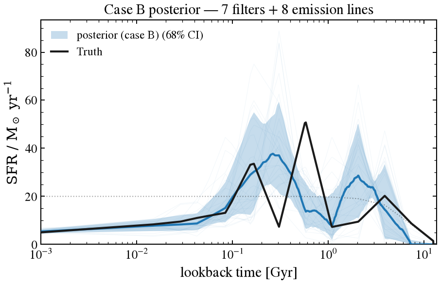
Read that figure carefully, because it shows the limit as well as the success. Below ~0.1 Gyr the posterior tracks the injected history and the band is narrow: that is the emission lines doing their work. Between 0.1 and 1 Gyr the band is wide, yet the truth still leaves it at the 0.3 Gyr trough and the 0.6 Gyr peak, so the posterior smooths over the bursts rather than resolving them. The chain’s split R-hat above 1.01 is a further reason to read the band as shape, not as a calibrated interval.
That is the concrete reason for the advice in the next section: quote integrated quantities, whose errors are dominated by the well-measured part of the history, rather than the star-formation rate in an individual age bin.
What to take away
1. Emission lines are the biggest single win, and extra filters are not. Adding 8 optical lines to the same 7 filters is what fixes the recent history: a factor of twelve below 15 Myr for the galaxy above (0.68 → 0.06 dex), and 0.37 → 0.10 dex as a median over three independent realizations. Widening the filter set instead, to a COSMOS-like 20 bands with medium bands included, leaves that number essentially unchanged. Broadband photometry integrates over the young light; the lines measure it. For an SDSS-like sample the spectrum is the whole game and extra filters add almost nothing.
2. The old mass budget comes from the continuum and the lines. In the galaxy above the fraction of mass formed more than 1 Gyr ago is 0.68 from photometry alone, 0.77 with lines and 0.85 with the spectrum, against a truth of 0.80: the photometry underestimates it by 0.12, and lines and spectrum land within about 0.05 of the truth on either side. The three-realization study gives the same ordering (truth 0.798; 0.758 photometry, 0.780 with lines, 0.804 with a spectrum), where the spectrum comes closest. The 4000 Å break and Balmer absorption carry that information beyond what a list of line fluxes holds.
3. Below 15 Myr, lines and a spectrum are equivalent; one galaxy cannot rank them. That equivalence is expected: the lines are the part of the spectrum carrying recent-SFH information, and over three realizations both give 0.10 dex. In the single galaxy above they score 0.06 and 0.10 dex, both far ahead of photometry alone (0.68 dex). The intermediate window (15 Myr – 1 Gyr) is noisier still: 0.39 dex from photometry, 0.26 with lines and 0.34 with the spectrum, a gap that one realization cannot separate, while the three-realization medians put lines and spectrum within 0.01 dex of each other and both ahead of photometry alone. Read the direction of these effects, not the ordering of one realization.
4. Report integrals, not per-node rates. The old population’s mass is well measured even where its per-node SFR is not constrained at all, which is why the mass-fraction panel is meaningful while a per-node comparison beyond 1 Gyr is not. Quote physically defined integrals (SFR averaged over 0–10 and 0–100 Myr, \(M_\star\), mass-weighted age) rather than the star-formation rate in an individual age bin.
5. More age bins do not mean more resolution. n_grid sets how smooth the field is, not how much the data can say: quadrupling it from 16 to 64 leaves the recovered information flat while tripling the dimension a sampler has to explore. This page uses n_grid=16, which keeps the dimension (25 here) small enough that HMC still behaves.
Scope of this demonstration
One galaxy, one burstiness (\(\sigma = 0.4\) dex), one redshift, and a pessimistic line signal-to-noise of 10. The population-level versions of these experiments (paired photometry-versus-lines contrasts, the burstiness ladder, and the n_grid sweep) live in scripts/field_sfh_recovery_study.py, which is where the multi-realization numbers quoted above come from:
python scripts/field_sfh_recovery_study.py --stage paired
python scripts/field_sfh_recovery_study.py --stage spectrum --n-seeds 15