Note
Go to the end to download the full example code.
Lyman-alpha emitter spectrum at z=6: IGM absorption and Lyα escape
High-redshift Lyα emitter at z=6 with young age (~10 Myr), low metallicity (Z~0.1 Z☉), and minimal dust. The observed-frame spectrum (7000–13000 Å) reveals the redshifted Lyα emission line at 8512 Å, the Lyman break at 6384 Å, characteristic IGM blue-wing absorption, and the rest-UV continuum. Demonstrates Lyα radiative transfer and reionization-era observability.
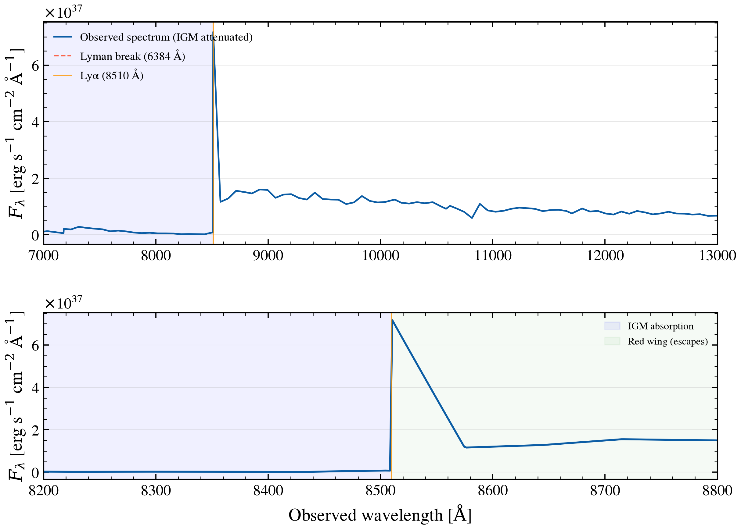
import os

os.environ["TF_CPP_MIN_LOG_LEVEL"] = "2"

import warnings

import jax
import matplotlib.pyplot as plt
import numpy as np

import tengri
from tengri.igm import igm_transmission
from tengri.plot import setup_style

setup_style()
warnings.filterwarnings("ignore", message=".*BakedInBackend.*")

# ============================================================================
# Physical Constants
# ============================================================================
C_AA_PER_S = 2.998e18  # Speed of light in Angstrom/second
LYMAN_ALPHA_REST = 1215.67  # Angstrom, rest-frame Lyα (vacuum)
LYMAN_BREAK_REST = 912.0  # Angstrom, Lyman series limit (hydrogen ionization edge)

# ============================================================================
# Model Setup: Young LAE at z=6
# ============================================================================
# Young star-forming galaxy with strong Lyα emission
# Uses bare-stellar SSP + Cue nebular to enable Lyα escape tracking

ssp = tengri.load_ssp("fsps_prsc_miles_chabrier")

model = tengri.SEDModel.build(
    ssp,
    sfh={
        "type": "dpl",
        "all_params": tengri.Fixed(tengri.DEFAULT),
        "tau_gyr": 0.01,  # Very young: 10 Myr timescale
        "log_total_mass": 7.5,  # Total mass ~3e7 Msun (SFR from tau_gyr duration)
        "alpha": 3.5,  # Rising early SFR
        "beta": 2.5,
    },  # Declining late SFR
    dust_attenuation={
        "law": "power_law",
        "type": "two_component",
        "all_params": tengri.Fixed(tengri.DEFAULT),
        "tau_diff": 0.02,  # Minimal diffuse dust
        "tau_bc": 0.05,
    },  # Minimal birth cloud dust
    neb={
        "type": "cue",
        "all_params": tengri.Fixed(tengri.DEFAULT),
        "logU": -2.5,  # Low ionization parameter
        "logZ_gas": -1.0,  # Low metallicity: Z ~ 0.1 Zsun
        "fesc": 0.1,  # Hydrogen ionizing photon escape
        "fesc_lya": 0.7,
    },  # Lyα escape fraction (realistic for LAE)
    igm={"type": "inoue14"},  # Inoue et al. 2014 IGM attenuation
    redshift=tengri.Fixed(6.0),
)

# Sample parameters
p = dict(model.spec.sample(jax.random.PRNGKey(42)))

# ============================================================================
# Observed-Frame Wavelength Grid and SED Prediction
# ============================================================================
z = 6.0
rest_to_obs = 1.0 + z

# Observed-frame grid: 7000–13000 Å (covers redshifted Lyα and continuum)
wave_obs_aa = np.linspace(7000.0, 13000.0, 3000)

# Predict rest-frame SED
out_rest = model.predict(p)
wave_rest = np.asarray(model.wavelengths)
sed_rest = np.asarray(out_rest.rest_sed())

# Map observed wavelengths back to rest-frame for interpolation
wave_rest_from_obs = wave_obs_aa / rest_to_obs
sed_obs_no_igm = np.interp(wave_rest_from_obs, wave_rest, sed_rest, left=0, right=0)

# Apply IGM transmission in observed frame
igm_trans = igm_transmission(wave_obs_aa, z_source=z)
sed_obs = sed_obs_no_igm * igm_trans

# Convert to f_λ (erg/s/cm^2/Å) for flux display
f_lam_obs = sed_obs * C_AA_PER_S / (wave_obs_aa**2)

# ============================================================================
# Key Features for Annotation
# ============================================================================
lya_obs_aa = LYMAN_ALPHA_REST * rest_to_obs
lyman_break_obs_aa = LYMAN_BREAK_REST * rest_to_obs

# ============================================================================
# Figure: Two-Panel Layout
# ============================================================================
fig, (ax_full, ax_lya) = plt.subplots(
    2, 1, figsize=(9.5, 6.5), gridspec_kw={"height_ratios": [2, 1.5], "hspace": 0.35}
)

# ---- Panel 1: Full spectrum (7000–13000 Å) ----
ax_full.plot(
    wave_obs_aa, f_lam_obs, color="C0", lw=1.3, label="Observed spectrum (IGM attenuated)"
)

# Lyman break annotation
ax_full.axvline(
    lyman_break_obs_aa,
    color="C3",
    lw=1.0,
    linestyle="--",
    alpha=0.7,
    label=f"Lyman break ({lyman_break_obs_aa:.0f} Å)",
)

# Lyα emission line annotation
ax_full.axvline(
    lya_obs_aa, color="C2", lw=1.2, linestyle="-", alpha=0.8, label=f"Lyα ({lya_obs_aa:.0f} Å)"
)

# Shade IGM blue-wing absorption region (wavelengths blueward of Lyα)
ax_full.axvspan(7000, lya_obs_aa, alpha=0.06, color="blue", zorder=1)

# Formatting
ax_full.set_ylabel(r"$F_\lambda$ [erg s$^{-1}$ cm$^{-2}$ Å$^{-1}$]")
ax_full.set_xlim(7000, 13000)
ax_full.legend(frameon=False, fontsize=9, loc="upper left")
ax_full.grid(True, alpha=0.3, which="major", axis="y")

# ---- Panel 2: Zoomed Lyα profile (8200–8800 Å) ----
zoom_lo, zoom_hi = 8200.0, 8800.0
mask_lya = (wave_obs_aa >= zoom_lo) & (wave_obs_aa <= zoom_hi)

ax_lya.plot(wave_obs_aa[mask_lya], f_lam_obs[mask_lya], color="C0", lw=1.5)
ax_lya.axvline(lya_obs_aa, color="C2", lw=1.2, linestyle="-", alpha=0.8)

# Asymmetric Lyα profile due to IGM: absorption on blue side, emission on red side
ax_lya.axvspan(zoom_lo, lya_obs_aa, alpha=0.06, color="blue", label="IGM absorption")
ax_lya.axvspan(lya_obs_aa, zoom_hi, alpha=0.04, color="green", label="Red wing (escapes)")

ax_lya.set_xlabel(r"Observed wavelength [$\mathrm{\AA}$]")
ax_lya.set_ylabel(r"$F_\lambda$ [erg s$^{-1}$ cm$^{-2}$ Å$^{-1}$]")
ax_lya.set_xlim(zoom_lo, zoom_hi)
ax_lya.legend(frameon=False, fontsize=8, loc="upper right")
ax_lya.grid(True, alpha=0.3, which="major", axis="y")

plt.savefig("plot_lae_spectrum_z6.png", dpi=150, bbox_inches="tight")
Total running time of the script: (0 minutes 5.486 seconds)