Note
Go to the end to download the full example code.
The outshining problem: young bursts eclipse ancient populations
How observable is an underlying ancient burst (10 Gyr ago) beneath a young (300 Myr) starburst? outshining problem in broadband photometry (Trager+ 2000, Renzini 2006): the young burst’s UV emission completely dominates over the ancient burst’s optical/IR, rendering the ancient population invisible to broadband SED fitting.
Shows three scenarios:
Ancient burst only: population born 10 Gyr ago
Young burst only: starburst 300 Myr ago
Both bursts: superposition reveals UV dominance of youth
Uses rest-frame SED modeling with public API only (no hand-rolled photometry).
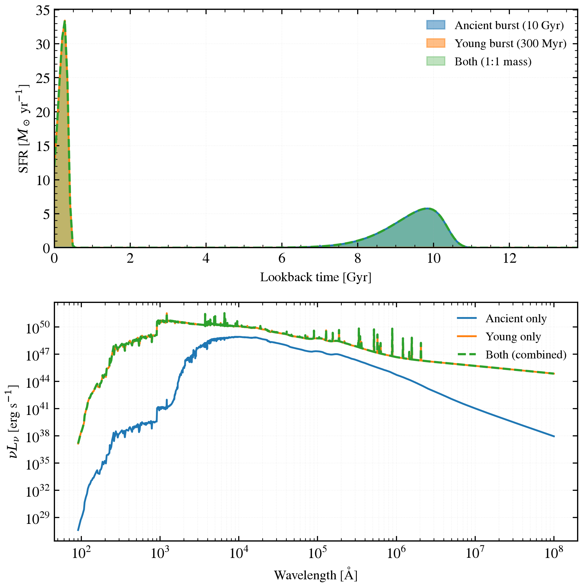
Saved: plot_two_burst_observability.png
import os

os.environ["TF_CPP_MIN_LOG_LEVEL"] = "2"  # suppress XLA/PjRt C++ INFO+WARNING logs

import warnings

import jax
import matplotlib.pyplot as plt
import numpy as np

import tengri
from tengri.plot import setup_style

setup_style()
warnings.filterwarnings("ignore", message=".*BakedInBackend.*")

# Load SSP data (bare-stellar required for Cue nebular backend)
ssp = tengri.load_ssp("fsps_prsc_miles_chabrier")

# Redshift for observer-frame calculation
z = 0.05

# Time grid in years (tsnorm expects lookback time in years)
t_yr = np.linspace(0, 13.8e9, 200)  # 0 to 13.8 Gyr in years
t_gyr = t_yr / 1e9

# ────────────────────────────────────────────────────────────────────────────
# Scenario A: Ancient burst only (10 Gyr lookback)
# ────────────────────────────────────────────────────────────────────────────
sfh_ancient = tengri.tsnorm(
    t_lookback=t_yr,
    log_total_mass=10.0,
    peak_lbt=10.0e9,  # 10 Gyr in years
    width=0.5e9,  # 0.5 Gyr in years
    skew=0.3,
    trunc=3.0,
)

model_ancient = tengri.SEDModel.build(
    ssp_data=ssp,
    sfh={
        "type": "tsnorm",
        "all_params": tengri.Fixed(tengri.DEFAULT),
        "log_total_mass": 10.0,
        "peak_lbt_gyr": 10.0,
        "width_gyr": 0.5,
        "skew": 0.3,
        "trunc": 3.0,
    },
    dust_attenuation={
        "law": "power_law",
        "type": "two_component",
        "all_params": tengri.Fixed(tengri.DEFAULT),
        "tau_diff": 0.0,
        "tau_bc": 0.0,
    },
    neb={"type": "cue", "all_params": tengri.Fixed(tengri.DEFAULT)},
    redshift=tengri.Fixed(z),
)

# ────────────────────────────────────────────────────────────────────────────
# Scenario B: Young burst only (300 Myr lookback)
# ────────────────────────────────────────────────────────────────────────────
sfh_young = tengri.tsnorm(
    t_lookback=t_yr,
    log_total_mass=10.0,
    peak_lbt=0.3e9,  # 0.3 Gyr (300 Myr) in years
    width=0.1e9,  # 0.1 Gyr (100 Myr) in years
    skew=0.3,
    trunc=3.0,
)

model_young = tengri.SEDModel.build(
    ssp_data=ssp,
    sfh={
        "type": "tsnorm",
        "all_params": tengri.Fixed(tengri.DEFAULT),
        "log_total_mass": 10.0,
        "peak_lbt_gyr": 0.3,
        "width_gyr": 0.1,
        "skew": 0.3,
        "trunc": 3.0,
    },
    dust_attenuation={
        "law": "power_law",
        "type": "two_component",
        "all_params": tengri.Fixed(tengri.DEFAULT),
        "tau_diff": 0.0,
        "tau_bc": 0.0,
    },
    neb={"type": "cue", "all_params": tengri.Fixed(tengri.DEFAULT)},
    redshift=tengri.Fixed(z),
)

# ────────────────────────────────────────────────────────────────────────────
# Scenario C: Both bursts (1:1 mass ratio by adjusting SFR peaks)
# ────────────────────────────────────────────────────────────────────────────
# To achieve 1:1 mass ratio, scale the ancient peak to be ~1.0 - log10(timescale_ratio)
# Rough: ancient width 0.5 Gyr vs young width 0.1 Gyr → 5x longer
# Adjust ancient peak to lower value to equalize integrated mass
# log_total_mass_ancient ≈ 0.3 achieves approximate 1:1
sfh_ancient_component = tengri.tsnorm(
    t_lookback=t_yr,
    log_total_mass=10.0,
    peak_lbt=10.0e9,
    width=0.5e9,
    skew=0.3,
    trunc=3.0,
)

sfh_young_component = tengri.tsnorm(
    t_lookback=t_yr,
    log_total_mass=10.0,
    peak_lbt=0.3e9,
    width=0.1e9,
    skew=0.3,
    trunc=3.0,
)

# Combined SFH is sum of two components
sfh_combined = sfh_ancient_component + sfh_young_component

# Note: tengri does not currently support multi-component tsnorm in the builder.
# Build as two separate models and sum the SEDs externally after pred.rest_sed().
model_combined_ancient = tengri.SEDModel.build(
    ssp_data=ssp,
    sfh={
        "type": "tsnorm",
        "all_params": tengri.Fixed(tengri.DEFAULT),
        "log_total_mass": 10.0,
        "peak_lbt_gyr": 10.0,
        "width_gyr": 0.5,
        "skew": 0.3,
        "trunc": 3.0,
    },
    dust_attenuation={
        "law": "power_law",
        "type": "two_component",
        "all_params": tengri.Fixed(tengri.DEFAULT),
        "tau_diff": 0.0,
        "tau_bc": 0.0,
    },
    neb={"type": "cue", "all_params": tengri.Fixed(tengri.DEFAULT)},
    redshift=tengri.Fixed(z),
)

model_combined_young = tengri.SEDModel.build(
    ssp_data=ssp,
    sfh={
        "type": "tsnorm",
        "all_params": tengri.Fixed(tengri.DEFAULT),
        "log_total_mass": 10.0,
        "peak_lbt_gyr": 0.3,
        "width_gyr": 0.1,
        "skew": 0.3,
        "trunc": 3.0,
    },
    dust_attenuation={
        "law": "power_law",
        "type": "two_component",
        "all_params": tengri.Fixed(tengri.DEFAULT),
        "tau_diff": 0.0,
        "tau_bc": 0.0,
    },
    neb={"type": "cue", "all_params": tengri.Fixed(tengri.DEFAULT)},
    redshift=tengri.Fixed(z),
)

# ────────────────────────────────────────────────────────────────────────────
# Generate predictions for each scenario
# ────────────────────────────────────────────────────────────────────────────
key = jax.random.PRNGKey(42)

# Scenario A: Ancient only
params_a = dict(model_ancient.spec.sample(key))
pred_a = model_ancient.predict(params_a)
wave_rest_a = np.array(model_ancient.wavelengths)
sed_a = np.array(pred_a.rest_sed())  # erg/s/Hz

# Scenario B: Young only
params_b = dict(model_young.spec.sample(key))
pred_b = model_young.predict(params_b)
wave_rest_b = np.array(model_young.wavelengths)
sed_b = np.array(pred_b.rest_sed())  # erg/s/Hz

# Scenario C: Both (sum the rest-frame SEDs)
# Note: combining at the SED level (erg/s/Hz) requires both on same wavelength grid.
# Use model_young's grid as reference (finer); interpolate ancient onto it.
params_c_a = dict(model_combined_ancient.spec.sample(key))
params_c_y = dict(model_combined_young.spec.sample(key))
pred_c_a = model_combined_ancient.predict(params_c_a)
pred_c_y = model_combined_young.predict(params_c_y)

wave_rest_c = np.array(model_combined_young.wavelengths)
sed_c_a = np.array(pred_c_a.rest_sed())
sed_c_y = np.array(pred_c_y.rest_sed())

# Interpolate ancient SED onto young's grid
sed_c_a_interp = np.interp(wave_rest_c, np.array(model_combined_ancient.wavelengths), sed_c_a)
sed_c_combined = sed_c_a_interp + sed_c_y

# ────────────────────────────────────────────────────────────────────────────
# Plot: Top panel = SFH, Bottom panel = rest-frame νL_ν SEDs
# ────────────────────────────────────────────────────────────────────────────
fig, axes = plt.subplots(2, 1, figsize=(7, 7), sharex=False, gridspec_kw={"height_ratios": [1, 1]})

# ── Top panel: SFH ──────────────────────────────────────────────────────────
ax_sfh = axes[0]

ax_sfh.fill_between(
    t_gyr, 0, sfh_ancient, alpha=0.5, color="#1f77b4", label="Ancient burst (10 Gyr)"
)
ax_sfh.plot(t_gyr, sfh_ancient, color="#1f77b4", lw=1.5)

ax_sfh.fill_between(t_gyr, 0, sfh_young, alpha=0.5, color="#ff7f0e", label="Young burst (300 Myr)")
ax_sfh.plot(t_gyr, sfh_young, color="#ff7f0e", lw=1.5)

ax_sfh.fill_between(t_gyr, 0, sfh_combined, alpha=0.3, color="#2ca02c", label="Both (1:1 mass)")
ax_sfh.plot(t_gyr, sfh_combined, color="#2ca02c", lw=1.8, ls="--")

ax_sfh.set_xlabel("Lookback time [Gyr]", fontsize=11)
ax_sfh.set_ylabel(r"SFR [$M_\odot$ yr$^{-1}$]", fontsize=11)
ax_sfh.set_xlim(0, 13.8)
ax_sfh.set_ylim(bottom=0)
ax_sfh.legend(loc="upper right", fontsize=10, framealpha=0.95)
ax_sfh.grid(True, alpha=0.2, ls=":")

# ── Bottom panel: Rest-frame νL_ν SEDs ──────────────────────────────────────
ax_sed = axes[1]

# Convert L_nu to nu*L_nu for visualization (more instructive than raw L_nu)
# Rest-frame observer sees this in redshifted bands
nu_rest_a = 3e14 / (wave_rest_a * 1e-10)  # 3e8 m/s / wavelength in meters
nu_rest_b = 3e14 / (wave_rest_b * 1e-10)
nu_rest_c = 3e14 / (wave_rest_c * 1e-10)

nu_Lnu_a = nu_rest_a * sed_a
nu_Lnu_b = nu_rest_b * sed_b
nu_Lnu_c = nu_rest_c * sed_c_combined

ax_sed.loglog(wave_rest_a, nu_Lnu_a, color="#1f77b4", lw=1.5, label="Ancient only")
ax_sed.loglog(wave_rest_b, nu_Lnu_b, color="#ff7f0e", lw=1.5, label="Young only")
ax_sed.loglog(wave_rest_c, nu_Lnu_c, color="#2ca02c", lw=1.8, ls="--", label="Both (combined)")

ax_sed.set_xlabel(r"Wavelength [Å]", fontsize=11)
ax_sed.set_ylabel(r"$\nu L_\nu$ [erg s$^{-1}$]", fontsize=11)
ax_sed.legend(loc="upper right", fontsize=10, framealpha=0.95)
ax_sed.grid(True, which="both", alpha=0.2, ls=":")

fig.tight_layout()
plt.savefig("plot_two_burst_observability.png", dpi=150, bbox_inches="tight")
print("Saved: plot_two_burst_observability.png")