Note
Go to the end to download the full example code.
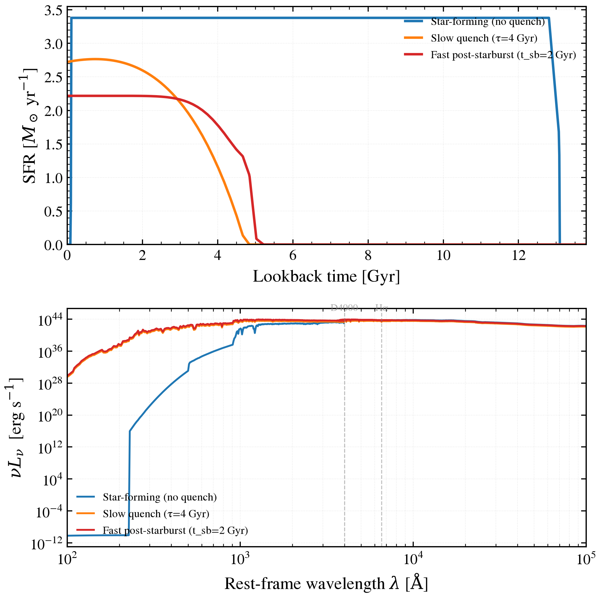
Quenching pathways: fast vs slow termination of star formation
Compare three star-formation histories representing distinct quenching scenarios: (1) Constantly star-forming (no quenching), (2) Slowly quenched exponential decay (tau=4 Gyr, peak 6 Gyr ago), and (3) Rapidly quenched post-starburst (truncated skew-normal, peak 2 Gyr ago, width 0.3 Gyr). The resulting rest-frame SEDs exhibit markedly different colors, equivalent widths (Hα), and spectral slopes, highlighting how quenching timescale imprints on observable photometry and spectroscopy.
/tengri/src/tengri/forward/sed_model.py:13787: SFHBeyondOldestTemplateWarning: The SSP grid's oldest template is 12.589 Gyr but the universe is 13.090 Gyr old at redshift 0.05. Stars formed in that gap are older than every template, so both age kernels assign them to the oldest one: the formed mass is conserved, and those stars carry the colors of a 12.589 Gyr population. Use a grid whose oldest template reaches 13.090 Gyr (e.g. MIST) to remove the approximation.
  return cls(
/tengri/src/tengri/forward/sed_model.py:13787: SFHBeyondOldestTemplateWarning: The SSP grid's oldest template is 12.589 Gyr but the universe is 13.090 Gyr old at redshift 0.05. Stars formed in that gap are older than every template, so both age kernels assign them to the oldest one: the formed mass is conserved, and those stars carry the colors of a 12.589 Gyr population. Use a grid whose oldest template reaches 13.090 Gyr (e.g. MIST) to remove the approximation.
  return cls(
/tengri/src/tengri/forward/sed_model.py:13787: SFHBeyondOldestTemplateWarning: The SSP grid's oldest template is 12.589 Gyr but the universe is 13.090 Gyr old at redshift 0.05. Stars formed in that gap are older than every template, so both age kernels assign them to the oldest one: the formed mass is conserved, and those stars carry the colors of a 12.589 Gyr population. Use a grid whose oldest template reaches 13.090 Gyr (e.g. MIST) to remove the approximation.
  return cls(
import os

os.environ["TF_CPP_MIN_LOG_LEVEL"] = "2"  # suppress XLA/PjRt C++ INFO+WARNING logs

import warnings

import jax
import jax.numpy as jnp
import matplotlib.pyplot as plt
import numpy as np

import tengri
from tengri.plot import setup_style

setup_style()
warnings.filterwarnings("ignore", message=".*BakedInBackend.*")
warnings.filterwarnings("ignore", message=".*deprecated.*")

ssp = tengri.load_ssp()

# --- Define three quenching scenarios ---
scenarios = [
    {
        "name": "Star-forming (no quench)",
        "sfh": {
            "type": "const",
            "all_params": tengri.Fixed(tengri.DEFAULT),
            "log_total_mass": 10.64,
            # start_frac is the lookback time to SF onset as a fraction of the age of
            # the universe at z = 0.05; 1.0 is formation at the Big Bang (13.09 Gyr ago).
            # end_gyr is lookback time to SF cessation (smaller number).
            # Star formation from the Big Bang until 0.1 Gyr ago.
            "start_frac": tengri.Fixed(1.0),
            "end_gyr": 0.1,
        },
        "color": "#1f77b4",
    },
    {
        "name": "Slow quench (τ=4 Gyr)",
        "sfh": {
            "type": "dexp",
            "all_params": tengri.Fixed(tengri.DEFAULT),
            "tau_gyr": 4.0,
            "log_total_mass": 10.0,
        },
        "color": "#ff7f0e",
    },
    {
        "name": "Fast post-starburst (t_sb=2 Gyr)",
        "sfh": {
            "type": "tsnorm",
            "all_params": tengri.Fixed(tengri.DEFAULT),
            "log_total_mass": 10.0,
            "peak_lbt_gyr": 2.0,
            "width_gyr": 0.3,
            "skew": 1.0,
            "trunc": 3.0,
        },
        "color": "#d62728",
    },
]

# --- Build models for each scenario ---
models = {}
params_dict = {}
for scenario in scenarios:
    model = tengri.SEDModel.build(
        ssp,
        sfh=scenario["sfh"],
        dust_attenuation={
            "law": "power_law",
            "type": "two_component",
            "all_params": tengri.Fixed(tengri.DEFAULT),
            "tau_diff": 0.15,
            "tau_bc": 0.3,
        },
        redshift=tengri.Fixed(0.05),
    )
    models[scenario["name"]] = model
    params_dict[scenario["name"]] = dict(model.spec.sample(jax.random.PRNGKey(42)))

# --- Compute SFH and SED predictions ---
sfh_data = {}
sed_data = {}

t_lookback = jnp.linspace(0, 13.8, 500)

for scenario in scenarios:
    name = scenario["name"]
    model = models[name]
    params = params_dict[name]

    # SFH predictions
    sfh_out = model.predict_sfh(params)
    sfh_data[name] = {
        "t_gyr": np.asarray(sfh_out["t_gyr"]),
        "sfr_mean": np.asarray(sfh_out["sfr_mean"]),
    }

    # Rest-frame SED predictions
    sed_out = model.predict(params)
    wave = np.asarray(model.wavelengths)
    nu = 2.998e18 / wave  # c in A/s -> frequency in Hz
    nu_l_nu = nu * np.asarray(sed_out.rest_sed())
    sed_data[name] = {"wave": wave, "nu_l_nu": nu_l_nu}

# --- Create two-panel figure ---
fig, axes = plt.subplots(2, 1, figsize=(7, 7))

# --- Top panel: SFH comparison ---
ax_sfh = axes[0]
for scenario in scenarios:
    name = scenario["name"]
    sfh = sfh_data[name]
    ax_sfh.plot(sfh["t_gyr"], sfh["sfr_mean"], label=name, color=scenario["color"], lw=2.0)

ax_sfh.set_xlabel("Lookback time [Gyr]")
ax_sfh.set_ylabel(r"SFR [$M_\odot$ yr$^{-1}$]")
ax_sfh.set_xlim(0, 13.8)
ax_sfh.set_ylim(0, None)
ax_sfh.legend(fontsize=9, frameon=False, loc="upper right")
ax_sfh.grid(alpha=0.3, linestyle=":", linewidth=0.5)

# --- Bottom panel: SED comparison (log-log) ---
ax_sed = axes[1]
for scenario in scenarios:
    name = scenario["name"]
    sed = sed_data[name]
    ax_sed.loglog(sed["wave"], sed["nu_l_nu"], label=name, color=scenario["color"], lw=1.5)

# Annotate key diagnostic features
ax_sed.axvline(6564.61, color="gray", linestyle="--", linewidth=0.8, alpha=0.5)  # H-alpha
ax_sed.axvline(4000, color="gray", linestyle="--", linewidth=0.8, alpha=0.5)  # D4000 break
ax_sed.text(6564.61, 1.2e46, "Hα", fontsize=8, ha="center", color="gray", alpha=0.7)
ax_sed.text(4000, 1.2e46, "D4000", fontsize=8, ha="center", color="gray", alpha=0.7)

ax_sed.set_xlim(100, 1e5)
ax_sed.set_xlabel(r"Rest-frame wavelength $\lambda$ [$\mathrm{\AA}$]")
ax_sed.set_ylabel(r"$\nu L_\nu$  [erg s$^{-1}$]")
ax_sed.legend(fontsize=9, frameon=False, loc="lower left")
ax_sed.grid(alpha=0.3, linestyle=":", linewidth=0.5, which="both")

fig.tight_layout()
plt.savefig("plot_quenching_pathway_compare.png", dpi=150, bbox_inches="tight")
Total running time of the script: (0 minutes 4.092 seconds)