Note
Go to the end to download the full example code.
Register and use a custom photometric filter
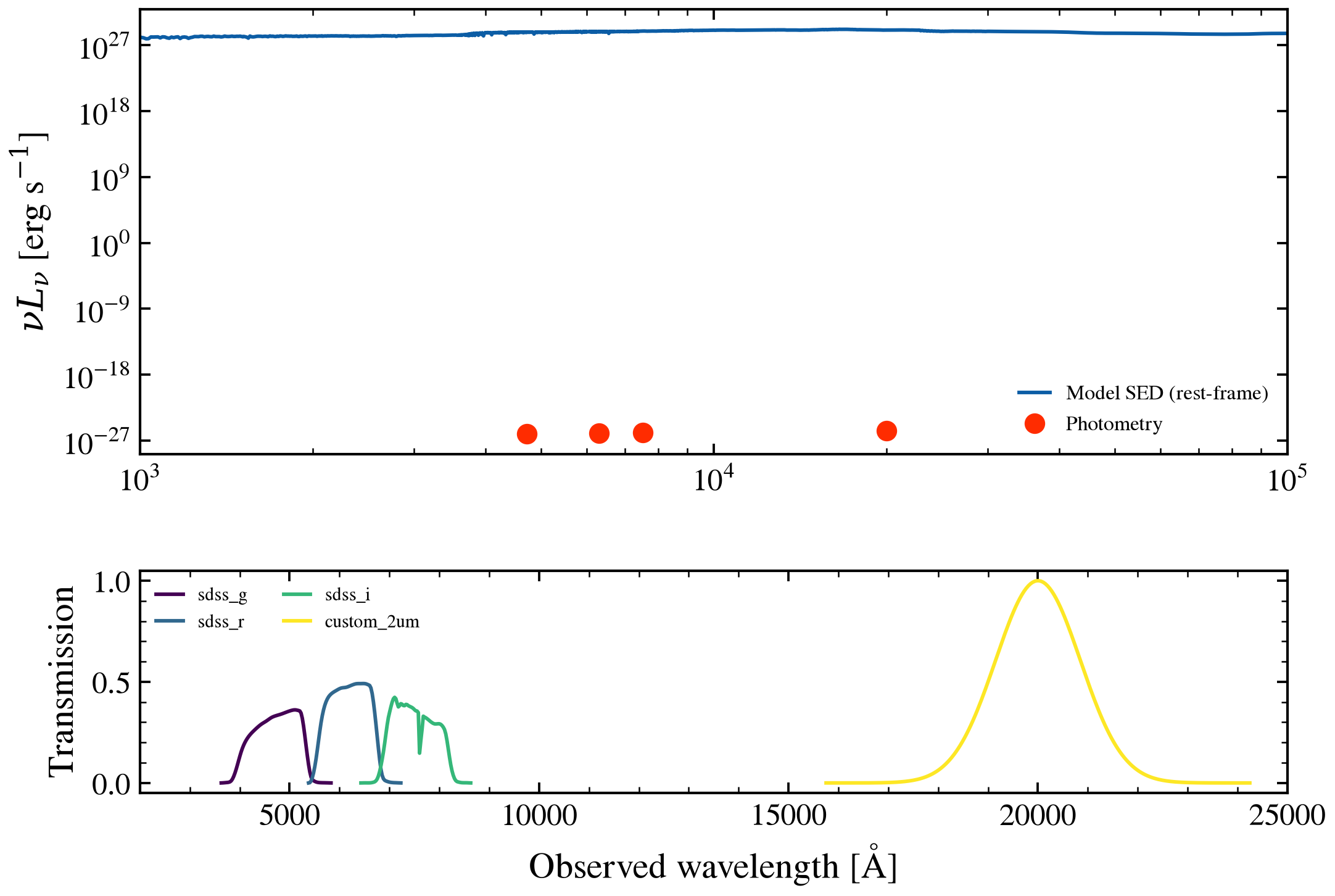
Build a FilterCurve from a Gaussian transmission profile and combine it with standard filters. The Photometry object merges them, then SEDModel predicts photometry on all bands at once — custom filters compose naturally with the standard library.
import os

os.environ["TF_CPP_MIN_LOG_LEVEL"] = "2"  # suppress XLA/PjRt C++ INFO+WARNING logs

import warnings

import jax.numpy as jnp
import matplotlib.pyplot as plt
import numpy as np

import tengri
from tengri import FilterCurve
from tengri.plot import setup_style

setup_style()
warnings.filterwarnings("ignore", message=".*BakedInBackend.*")

ssp = tengri.load_ssp()

# Build a synthetic Gaussian filter at 2 μm (20000 Å with 2000 Å FWHM)
wave_center = 20000.0
fwhm = 2000.0
sigma = fwhm / (2 * np.sqrt(2 * np.log(2)))
wave_grid = np.linspace(wave_center - 5 * sigma, wave_center + 5 * sigma, 200)
trans_curve = np.exp(-0.5 * ((wave_grid - wave_center) / sigma) ** 2)

custom_filter = FilterCurve(
    wave=jnp.array(wave_grid), trans=jnp.array(trans_curve), name="custom_2um"
)

# Combine with standard SDSS
sdss_phot = tengri.Photometry.from_names(["sdss_g", "sdss_r", "sdss_i"])
all_filters = [*sdss_phot.filters, custom_filter]
all_names = [*sdss_phot.names, "custom_2um"]
phot = tengri.Photometry(filters=tuple(all_filters), names=tuple(all_names))

# Build model using the nested-dict API
obs = tengri.Observation(photometry=phot)
model = tengri.SEDModel.build(
    ssp,
    observation=obs,
    sfh={
        "type": "tsnorm",
        "all_params": tengri.Fixed(tengri.DEFAULT),
        "log_total_mass": 10.0,
        "peak_lbt_gyr": 2.0,
        "width_gyr": 1.5,
        "skew": 0.2,
        "trunc": 5.0,
    },
    dust_attenuation={
        "law": "power_law",
        "type": "two_component",
        "all_params": tengri.Fixed(tengri.DEFAULT),
        "tau_bc": 0.1,
        "tau_diff": 0.2,
        "slope": -0.7,
    },
    redshift=tengri.Fixed(0.05),
)

# Predict SED and photometry
params = dict(model.spec.sample(tengri.jax.random.PRNGKey(0)))
sed_result = model.predict(params)
phot_flux = np.array(model.predict_photometry(params))
phot_wave = np.array([float(jnp.mean(w)) for w in phot.filter_waves])

# Plot: SED with photometry and filter responses
fig, (ax_sed, ax_filters) = plt.subplots(
    2, 1, figsize=(8.0, 5.5), sharex=False, gridspec_kw={"height_ratios": [2, 1], "hspace": 0.35}
)

# Top: SED + photometric points
wave_rest = np.asarray(model.wavelengths)
sed_rest = np.asarray(sed_result.rest_sed())
ax_sed.loglog(wave_rest, sed_rest, color="C0", lw=1.4, label="Model SED (rest-frame)")
ax_sed.plot(phot_wave, phot_flux, "o", color="C3", ms=7, label="Photometry", zorder=10)
ax_sed.set_ylabel(r"$\nu L_\nu$ [erg s$^{-1}$]")
ax_sed.legend(frameon=False, fontsize=8, loc="lower right")
ax_sed.set_xlim(1e3, 1e5)

# Bottom: Filter transmission curves
colors = plt.cm.viridis(np.linspace(0, 1, len(phot.names)))
for i, (fname, wave_filt, trans_filt) in enumerate(
    zip(phot.names, phot.filter_waves, phot.filter_trans)
):
    ax_filters.plot(wave_filt, trans_filt, color=colors[i], lw=1.4, label=fname)

ax_filters.set_xlabel(r"Observed wavelength [Å]")
ax_filters.set_ylabel("Transmission")
ax_filters.legend(frameon=False, ncol=2, fontsize=7)
ax_filters.set_xlim(2e3, 2.5e4)

plt.savefig("plot_recipe_custom_filter.png", dpi=150, bbox_inches="tight")