Note
Go to the end to download the full example code.
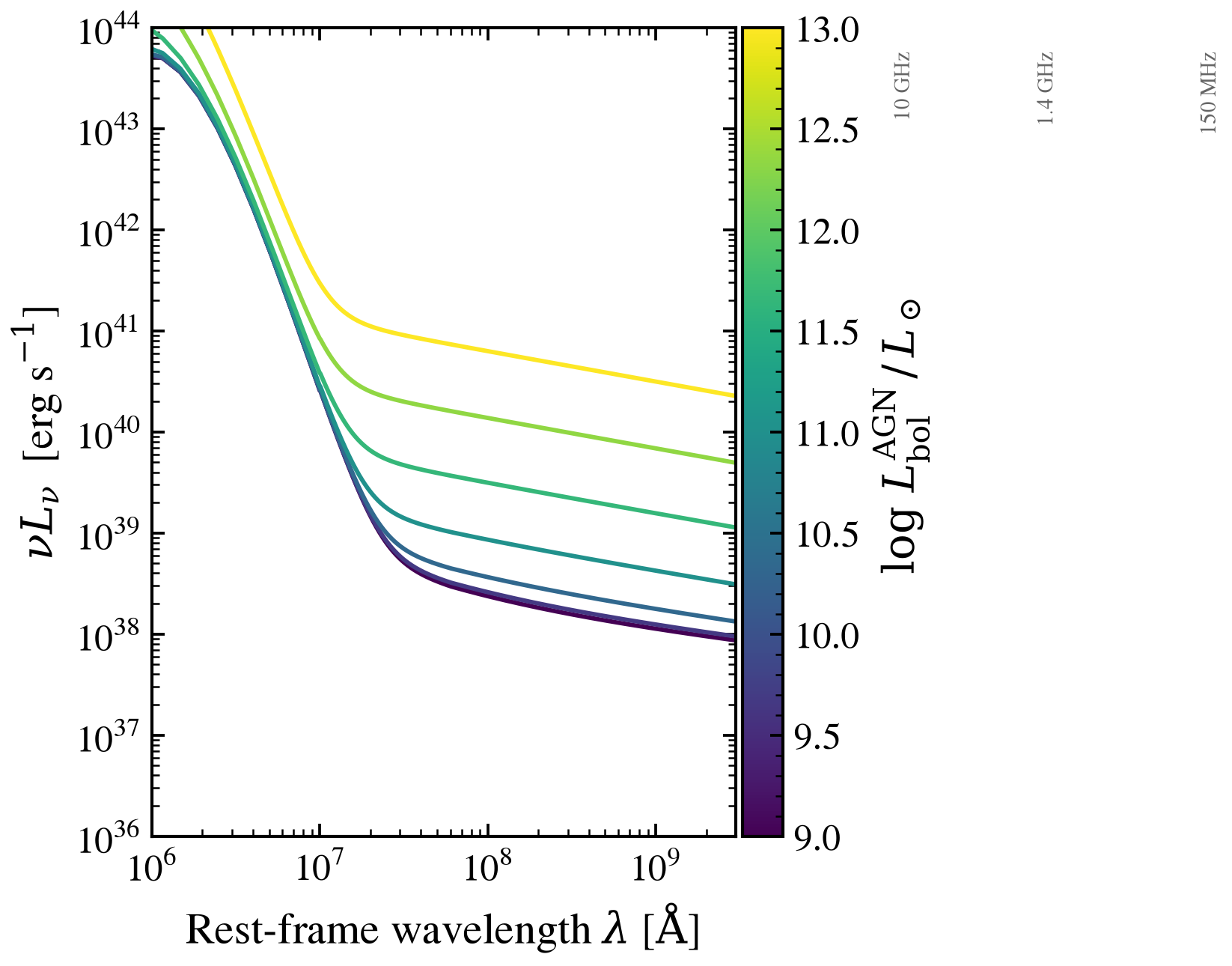
Radio SED response to AGN bolometric luminosity
At fixed host (constant SFR = 3 M☉/yr, Condon-92 synchrotron +
free-free) we sweep the composable AGN’s bolometric luminosity
agn_log_lbol from 9 to 13 (in log L_sun). The host alone produces
a power-law GHz continuum; the AGN superposes a flatter-spectrum jet
component that takes over above log L_bol ≳ 11.5 — the classic
radio-loud / radio-quiet division emerges from this competition.
This is the figure that motivates separating SF-driven from AGN-driven radio in unresolved sources (Best+2005, Pracy+2016).
import os

os.environ["TF_CPP_MIN_LOG_LEVEL"] = "2"  # suppress XLA/PjRt C++ INFO+WARNING logs

import warnings

import jax
import jax.numpy as jnp
import matplotlib as mpl
import matplotlib.pyplot as plt
import numpy as np

import tengri
from tengri.plot import setup_style

setup_style()
warnings.filterwarnings("ignore", message=".*BakedInBackend.*")

C_AA_PER_S = 2.998e18

log_lbol_grid = np.linspace(9.0, 13.0, 7)
norm = mpl.colors.Normalize(vmin=log_lbol_grid.min(), vmax=log_lbol_grid.max())
cmap = plt.get_cmap("viridis")

SFH = {
    "type": "const",
    "all_params": tengri.Fixed(tengri.DEFAULT),
    "log_total_mass": 10.61,
    "start_gyr": 13.0,
    "end_gyr": 0.0,
}
DUST = {
    "law": "power_law",
    "type": "two_component",
    "all_params": tengri.Fixed(tengri.DEFAULT),
    "tau_diff": 0.3,
    "tau_bc": 0.5,
}
# dale2014_cigale: this example enables the radio component, and plain
# dale2014 embeds its own SF radio continuum — the pair is refused at
# build as a double-count (#1970).
DUST_EMISSION = {"type": "dale2014_cigale", "all_params": tengri.Fixed(tengri.DEFAULT)}

ssp = tengri.load_ssp()
model = tengri.SEDModel.build(
    ssp,
    sfh=SFH,
    dust_attenuation=DUST,
    dust_emission=DUST_EMISSION,
    agn={
        "disc": {"type": "qsogen", "all_params": tengri.Fixed(tengri.DEFAULT)},
        "torus": {"type": "skirtor", "all_params": tengri.Fixed(tengri.DEFAULT)},
        "all_params": tengri.Fixed(tengri.DEFAULT),
        "log_lbol": tengri.Uniform(8.0, 14.0),
        "lum_ratio": 1.0,
    },
    radio={
        "sf": {"type": "bell2003"},
        "agn": {"type": "powerlaw"},
        "all_params": tengri.Fixed(tengri.DEFAULT),
    },
    redshift=tengri.Fixed(0.05),
)
baseline = dict(model.spec.sample(jax.random.PRNGKey(0)))

fig, ax = plt.subplots(figsize=(7.0, 4.6))
for log_lbol in log_lbol_grid:
    out = model.predict({**baseline, "agn_log_lbol": jnp.float64(log_lbol)})
    wave = np.asarray(model.wavelengths)
    nu_l_nu = C_AA_PER_S / wave * np.asarray(out.rest_sed())
    ax.loglog(wave, nu_l_nu, color=cmap(norm(log_lbol)), lw=1.4)

ax.set(
    xlim=(1e6, 3e9),
    ylim=(1e36, 1e44),
    xlabel=r"Rest-frame wavelength $\lambda$ [$\mathrm{\AA}$]",
    ylabel=r"$\nu L_\nu$  [erg s$^{-1}$]",
)
for nu_ghz, name in [(0.150, "150 MHz"), (1.4, "1.4 GHz"), (10.0, "10 GHz")]:
    lam = 2.998e10 / (nu_ghz * 1.0e9) * 1.0e10
    ax.axvline(lam, color="0.65", lw=0.4, ls=":")
    ax.text(
        lam,
        0.97,
        name,
        transform=ax.get_xaxis_transform(),
        fontsize=7,
        color="0.4",
        ha="center",
        rotation=90,
        va="top",
    )

cbar = fig.colorbar(plt.cm.ScalarMappable(norm=norm, cmap=cmap), ax=ax, pad=0.01)
cbar.set_label(r"$\log\,L_{\rm bol}^{\rm AGN}\,/\,L_\odot$")

fig.tight_layout()
plt.savefig("plot_radio_vs_agn_lbol.png", dpi=150, bbox_inches="tight")