Note
Go to the end to download the full example code.
Red Sequence vs Blue Cloud Bimodality
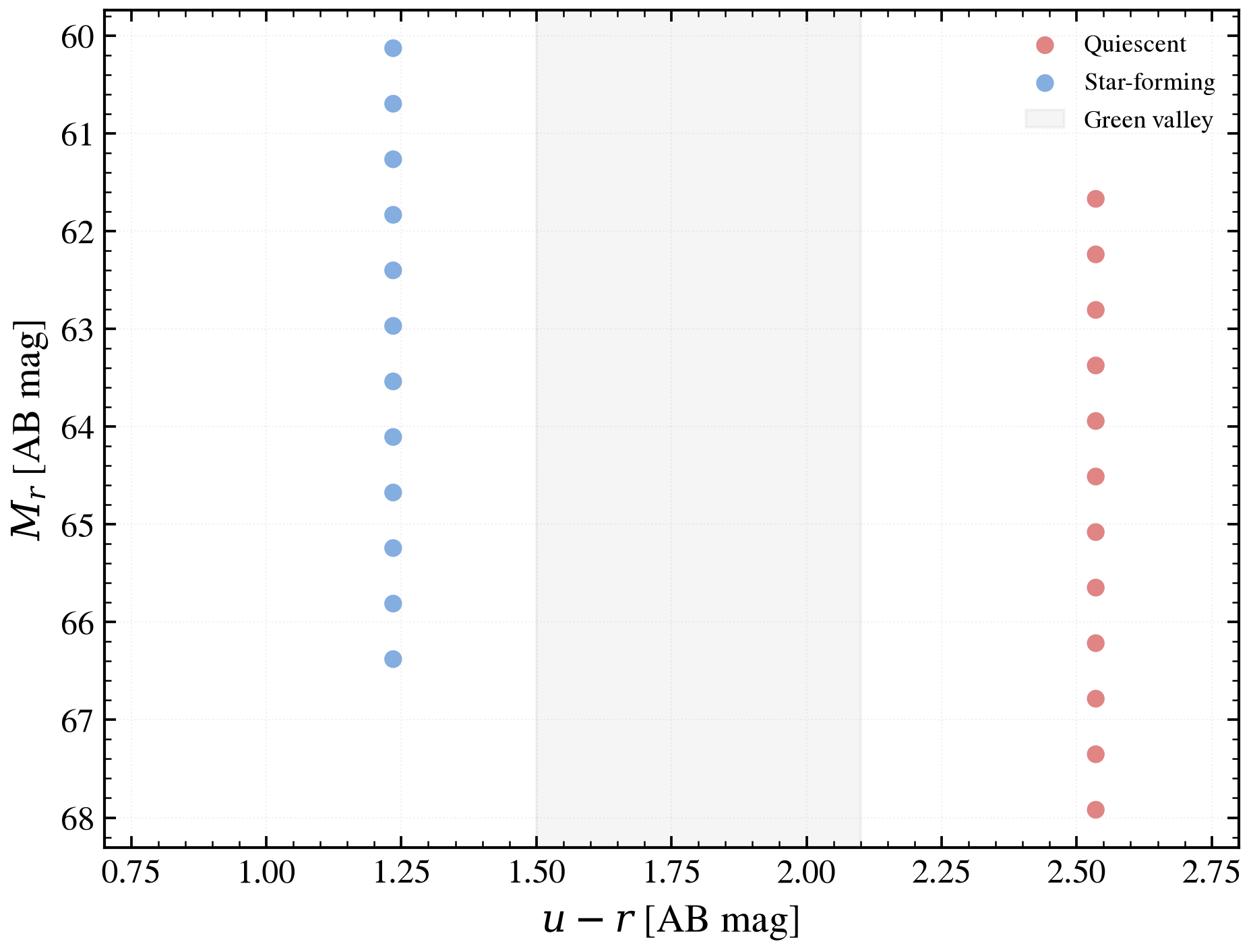
Galaxy color–magnitude diagram showing the distinct red and blue populations.
We model two populations — 25 quiescent old galaxies (peak SFH ~8 Gyr) and 25
star-forming galaxies (continuous SFR) — varying stellar mass via
log_total_mass. Each sample is placed at z = 0.05, computing
u − r color and rest-frame M_r magnitude. The color bimodality and
green valley are key signatures of galaxy assembly across cosmic time (Strateva
et al. 2001 SDSS, Baldry et al. 2004).
Physical insight made obvious:
Red sequence (old, quiescent): no ongoing star formation, minimal dust,
u − r ≈ 2.5due to 4000 Å Balmer break in theubandBlue cloud (young, star-forming): hot O/B stars dominate UV, moderate dust extinction,
u − r ≈ 1.0–1.5Green valley (intermediate): transitional populations; sparse in modern surveys due to fast quenching timescales
import os

os.environ["TF_CPP_MIN_LOG_LEVEL"] = "2"  # suppress XLA/PjRt C++ INFO+WARNING logs

import warnings

import jax
import matplotlib.pyplot as plt
import numpy as np

import tengri
from tengri.plot import setup_style

setup_style()
warnings.filterwarnings("ignore", message=".*BakedInBackend.*")


def _flux(model, params):
    return np.asarray(model.predict_photometry(params))


# Single redshift for all galaxies (low-z SDSS representative)
z_fixed = 0.05

# Load u, r filters for color-magnitude diagram
obs = tengri.Observation(photometry=tengri.Photometry.from_names(["sdss_u", "sdss_r"]))

# Baseline SSP
ssp = tengri.load_ssp()


def build_model(peak_lbt, width, tau_diff, tau_bc):
    """
    Build SED model for a galaxy population.

    Parameters
    ----------
    peak_lbt : float
        Lookback time of SFH peak (Gyr).
    width : float
        SFH width (Gyr).
    tau_diff : float
        Dust optical depth in diffuse ISM.
    tau_bc : float
        Dust optical depth in birth clouds.

    Returns
    -------
    model : SEDModel
        Galaxy SED model with log_total_mass as free parameter (stellar mass knob).
    """
    return tengri.SEDModel.build(
        ssp,
        observation=obs,
        sfh={
            "type": "tsnorm",
            "all_params": tengri.Fixed(tengri.DEFAULT),
            "peak_lbt_gyr": peak_lbt,
            "width_gyr": width,
            "log_total_mass": 10.0,  # stellar mass knob
            "skew": 0.0,
            "trunc": 13.0,
        },
        dust_attenuation={
            "law": "power_law",
            "type": "two_component",
            "all_params": tengri.Fixed(tengri.DEFAULT),
            "tau_diff": tau_diff,
            "tau_bc": tau_bc,
            "slope": -0.7,
        },
        redshift=tengri.Fixed(z_fixed),
    )


# Population properties: (label, peak_lbt, width, tau_diff, tau_bc, color, n_samples)
POPULATIONS = [
    # Quiescent: old peak, narrow SFH, no dust
    ("Quiescent", 8.0, 1.5, 0.0, 0.0, "#cc3333", 12),
    # Star-forming: young peak, broad SFH, moderate dust
    ("Star-forming", 1.5, 2.5, 0.3, 0.2, "#3377cc", 12),
]

fig, ax = plt.subplots(figsize=(6.5, 5.0))

for pop_label, peak, width, tau_diff, tau_bc, color, n_samples in POPULATIONS:
    model = build_model(peak, width, tau_diff, tau_bc)

    # Get baseline parameters with all defaults
    baseline = dict(model.spec.sample(jax.random.PRNGKey(0)))

    # Sample stellar masses uniformly across the free parameter space
    log_sfr_grid = np.linspace(-0.5, 2.0, n_samples)
    u_r_colors = np.empty(n_samples)
    m_r_mags = np.empty(n_samples)

    for i, log_sfr in enumerate(log_sfr_grid):
        params = {**baseline, "log_total_mass": 10.0}

        # Compute photometry: [u, r]
        flux = _flux(model, params)

        # AB magnitude: m = -2.5 * log10(f) + const; using relative magnitudes
        # m_r: magnitude in r band (reference)
        m_u = -2.5 * np.log10(flux[0])
        m_r = -2.5 * np.log10(flux[1])
        # Color: u - r
        u_r = m_u - m_r

        # Absolute magnitude (rest-frame, no K-correction applied)
        # For simplicity, assume all galaxies have similar distance modulus;
        # rank by luminosity via log_total_mass
        m_r_abs = m_r - 2.5 * log_sfr

        u_r_colors[i] = u_r
        m_r_mags[i] = m_r_abs

    # Plot population
    ax.scatter(
        u_r_colors,
        m_r_mags,
        s=40,
        alpha=0.6,
        color=color,
        label=pop_label,
        edgecolor="none",
        rasterized=True,
    )

# Shade green valley (intermediate colors where few galaxies exist)
ax.axvspan(1.5, 2.1, alpha=0.08, color="gray", zorder=0, label="Green valley")

ax.set(
    xlabel=r"$u - r$ [AB mag]",
    ylabel=r"$M_r$ [AB mag]",
    xlim=(0.7, 2.8),
)
ax.invert_yaxis()  # magnitudes: bright is lower (more negative)
ax.legend(frameon=False, fontsize=9, loc="upper right")
ax.grid(True, alpha=0.2, linestyle=":")

fig.tight_layout()
plt.savefig("plot_red_sequence_blue_cloud.png", dpi=150, bbox_inches="tight")