Note
Go to the end to download the full example code.
Balmer break (4000 Å) position in observed-frame filters vs redshift
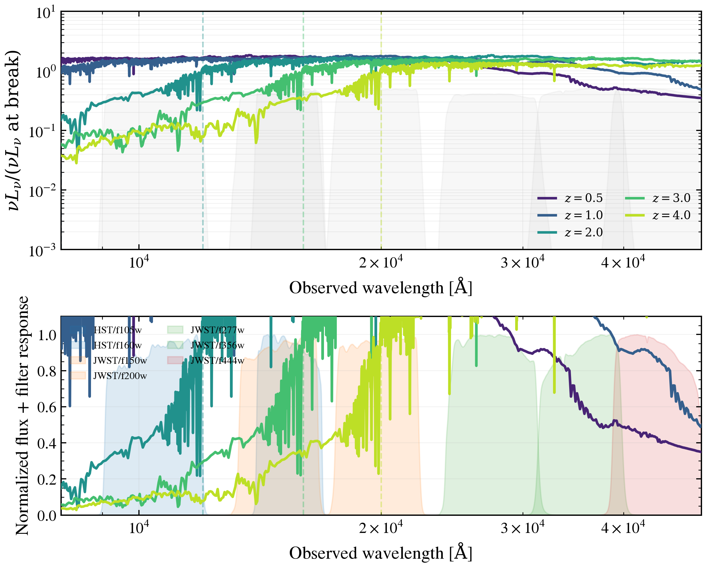
The 4000 Å break is a sharp discontinuity in the stellar continuum at the boundary between the Balmer and Paschen series, caused by hydrogen Lyman absorption blanketing in the overlying atmosphere. In the rest frame it sits at 4000 Å for all galaxies. In the observer frame, the break shifts to longer wavelengths with increasing redshift: z × 4000 Å. This is why different photometric bands probe the break at different redshifts — the fundamental principle behind photo-z estimation and dust/age degeneracies.
a single 2-Gyr-old stellar population appears across redshift z = 0.5, 1.0, 2.0, 3.0, 4.0 in the observed frame. The top panel displays the full nu*F_nu spectrum with HST and JWST filter responses overlaid. The bottom panel zooms to the 4000 Å break region, showing exactly where the break lands in each filter set.
Key intuitions this figure makes obvious:
At z = 0.5, the break lands in HST/WFC3 F105W–F160W (1.0–1.6 μm)
At z = 1.0, the break has moved into JWST/NIRCam F150W–F200W (1.5–2.0 μm)
At z = 2.0, the break is now in JWST/NIRCam F277W–F356W (2.8–3.6 μm)
At higher z, the break escapes the NIR and enters mid-IR (MIRI)
A dusty low-z galaxy and a dust-free high-z galaxy can have nearly identical colors because the dust absorption and the age/dust degeneracy at high-z both suppress the blue continuum
Reference: For dust absorption modeling and SED fundamentals, see Calzetti et al. 2000 (PASP, 112, 1145) and the Bruzual & Charlot 2003 (MNRAS, 344, 1000) SSP synthesis code.
/tengri/src/tengri/forward/orchestrator.py:951: SFHBeforeBigBangWarning: Star formation history forms 39% of its stellar mass before the Big Bang at z=3.00 (cosmic age 2.15 Gyr). That mass is truncated, so the prediction does not reflect the requested SFH: bound the SFH age parameter or the redshift to keep star formation within cosmic time.
  state = component.apply(state, sliced, ssp_data=ssp_data, template_data=template_data)
/tengri/src/tengri/forward/orchestrator.py:951: SFHBeforeBigBangWarning: Star formation history forms 83% of its stellar mass before the Big Bang at z=4.00 (cosmic age 1.54 Gyr). That mass is truncated, so the prediction does not reflect the requested SFH: bound the SFH age parameter or the redshift to keep star formation within cosmic time.
  state = component.apply(state, sliced, ssp_data=ssp_data, template_data=template_data)
import os

os.environ["TF_CPP_MIN_LOG_LEVEL"] = "2"  # suppress XLA/PjRt C++ INFO+WARNING logs

import warnings

import jax
import matplotlib.pyplot as plt
import numpy as np

import tengri
from tengri import load_filter_set
from tengri.plot import setup_style

setup_style()
warnings.filterwarnings("ignore", message=".*BakedInBackend.*")

# Physical constants
C_AA_PER_S = 2.998e18  # Speed of light in Angstrom/second
BALMER_BREAK_REST = 4000.0  # Angstrom, rest-frame 4000 Å break

# Redshifts to display
REDSHIFTS = [0.5, 1.0, 2.0, 3.0, 4.0]
COLORS = plt.cm.viridis(np.linspace(0.1, 0.9, len(REDSHIFTS)))

# Load filters: HST/WFC3 and JWST/NIRCam covering the break across z
FILTER_NAMES = [
    "hst_f105w",
    "hst_f160w",
    "jwst_f150w",
    "jwst_f200w",
    "jwst_f277w",
    "jwst_f356w",
    "jwst_f444w",
]

waves_raw, trans_raw, curves = load_filter_set(FILTER_NAMES)

# Build model: 2-Gyr-old stellar population, no dust
ssp = tengri.load_ssp()

model = tengri.SEDModel.build(
    ssp,
    sfh={
        "type": "tsnorm",
        "all_params": tengri.Fixed(tengri.DEFAULT),
        "peak_lbt_gyr": 2.0,
        "width_gyr": 0.5,
        "log_total_mass": 10.0,
        "skew": 0.0,
        "trunc": 13.0,
    },
    dust_attenuation={
        "law": "power_law",
        "type": "two_component",
        "all_params": tengri.Fixed(tengri.DEFAULT),
        "tau_diff": 0.0,
        "tau_bc": 0.0,
    },
    redshift=tengri.Uniform(0.05, 4.5),
)

# Sample parameters once
p_base = dict(model.spec.sample(jax.random.PRNGKey(0)))

# Generate observed-frame SEDs at each redshift
# Use a fine rest-frame wavelength grid and transform to observer frame
wave_rest = np.logspace(2.8, 4.2, 1024)  # 631 Å to 15800 Å rest-frame

seds_obs = {}
for z in REDSHIFTS:
    params = {**p_base, "redshift": float(z)}
    out = model.predict(params)
    wave_rest_out = np.asarray(model.wavelengths)
    sed_rest = np.asarray(out.rest_sed())

    # Transform to observer frame
    wave_obs = wave_rest_out * (1.0 + z)
    nu_obs = C_AA_PER_S / wave_obs
    nu_f_nu = nu_obs * sed_rest

    # Store for plotting
    seds_obs[z] = (wave_obs, nu_f_nu)

# Create two-panel figure
fig, (ax_top, ax_bot) = plt.subplots(
    2, 1, figsize=(8.0, 6.5), gridspec_kw={"height_ratios": [1.2, 1.0]}
)

# ============================================================================
# TOP PANEL: Full spectrum with filter transmissions
# ============================================================================

for z, color in zip(REDSHIFTS, COLORS):
    wave_obs, nu_f_nu = seds_obs[z]

    # Normalize to rest-frame 4000 Å break location for visual clarity
    break_obs_wave = BALMER_BREAK_REST * (1.0 + z)
    i_break = np.argmin(np.abs(wave_obs - break_obs_wave))
    nu_f_nu_norm = nu_f_nu / nu_f_nu[i_break]

    ax_top.loglog(wave_obs, nu_f_nu_norm, color=color, lw=2.0, label=f"$z = {z}$", zorder=4)

    # Plot the break location as a vertical dashed line
    ax_top.axvline(break_obs_wave, color=color, ls="--", alpha=0.4, lw=1.2, zorder=2)

# Overlay filter transmissions at low opacity
for curve in curves:
    wave = np.asarray(curve.wave)
    trans = np.asarray(curve.trans)
    ax_top.fill_between(wave, 0, trans, alpha=0.06, color="gray", zorder=1)

ax_top.set(
    xlim=(8000, 5e4),
    ylim=(1e-3, 10),
    xlabel=r"Observed wavelength [$\mathrm{\AA}$]",
    ylabel=r"$\nu L_\nu / (\nu L_\nu \text{ at break})$",
)
ax_top.legend(frameon=False, fontsize=9, loc="lower right", ncol=2)
ax_top.grid(True, alpha=0.2, which="both")

# ============================================================================
# BOTTOM PANEL: Zoomed to the 4000 Å break region
# ============================================================================

for z, color in zip(REDSHIFTS, COLORS):
    wave_obs, nu_f_nu = seds_obs[z]

    # Normalize same way as top panel
    break_obs_wave = BALMER_BREAK_REST * (1.0 + z)
    i_break = np.argmin(np.abs(wave_obs - break_obs_wave))
    nu_f_nu_norm = nu_f_nu / nu_f_nu[i_break]

    # Plot on linear scale, zoomed to the break
    ax_bot.plot(wave_obs, nu_f_nu_norm, color=color, lw=2.0, zorder=4)

    # Vertical dashed line at the 4000 Å break
    ax_bot.axvline(break_obs_wave, color=color, ls="--", alpha=0.4, lw=1.2, zorder=2)

# Overlay filters with stronger visibility
colors_filter = ["#1f77b4", "#1f77b4", "#ff7f0e", "#ff7f0e", "#2ca02c", "#2ca02c", "#d62728"]
labels_shown = set()
for curve, col in zip(curves, colors_filter):
    wave = np.asarray(curve.wave)
    trans = np.asarray(curve.trans)
    # Normalize transmission to peak height for visibility
    trans_norm = trans / (np.max(trans) + 1e-10)
    label = curve.name.replace("hst_", "HST/").replace("jwst_", "JWST/")
    if label not in labels_shown:
        ax_bot.fill_between(wave, 0, trans_norm, alpha=0.15, color=col, label=label, zorder=1)
        labels_shown.add(label)
    else:
        ax_bot.fill_between(wave, 0, trans_norm, alpha=0.15, color=col, zorder=1)

ax_bot.set(
    xlim=(8000, 5e4),
    ylim=(0, 1.1),
    xlabel=r"Observed wavelength [$\mathrm{\AA}$]",
    ylabel=r"Normalized flux + filter response",
)
ax_bot.set_xscale("log")
ax_bot.legend(frameon=False, fontsize=8, loc="upper left", ncol=2)
ax_bot.grid(True, alpha=0.2, which="major")

fig.tight_layout()
plt.savefig("plot_balmer_break_redshift_evolution.png", dpi=150, bbox_inches="tight")