Note
Go to the end to download the full example code.
Strong-line gas-phase metallicity diagnostics
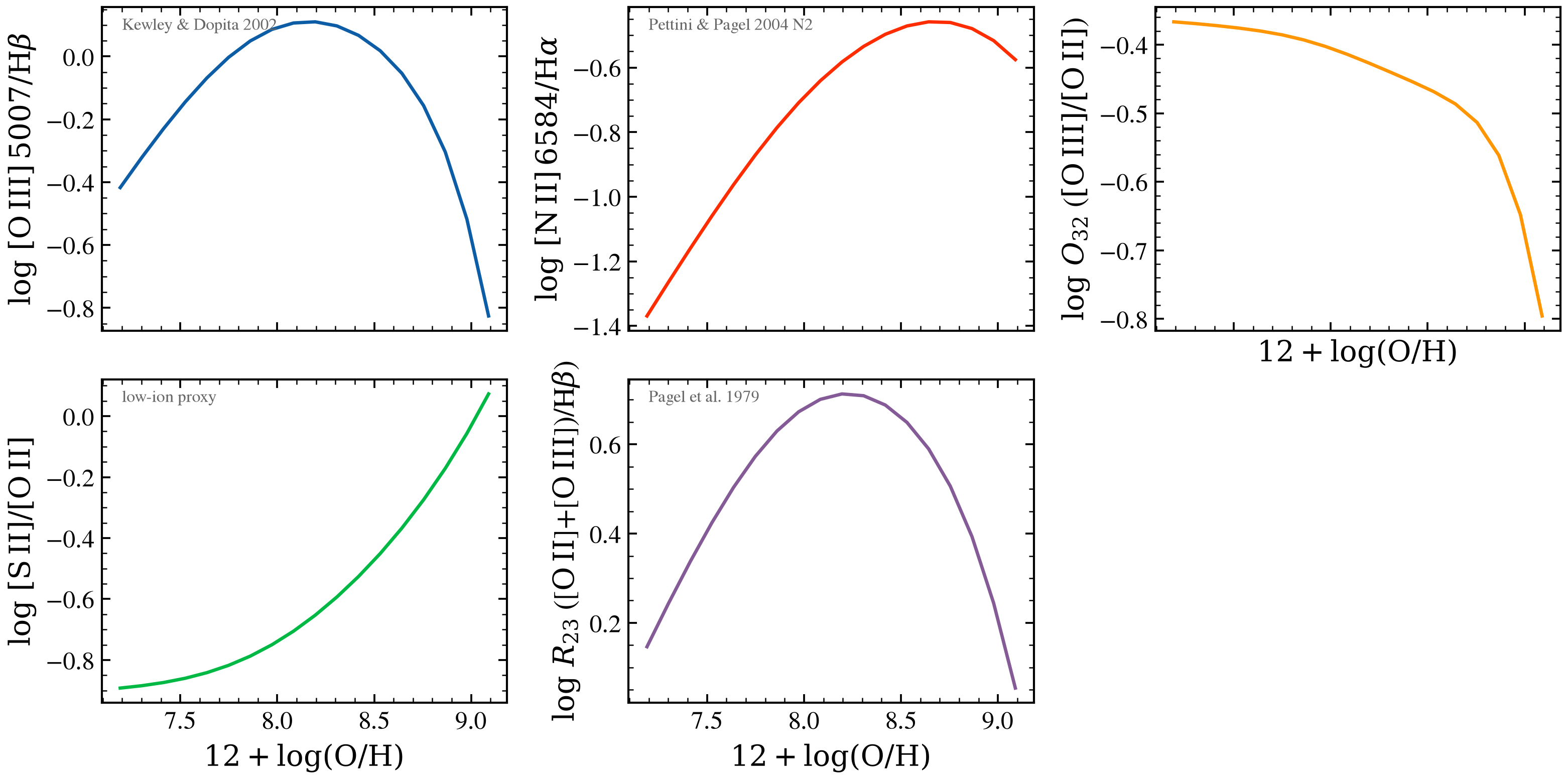
Five widely-used optical strong-line metallicity diagnostics
evaluated across the Cue logZ_gas prior. Each one carries a
different systematic — Pettini & Pagel 2004 O3N2 saturates at high
Z, the R23 ratio is double-valued (Pagel+1979), N2 (Marino+2013) is monotonic
but small dynamic range, the [O III]/[O II] diagnostic tracks ionization,
and [S II]/[O II] is a low-ion proxy.
This is the diagnostic family every observer chooses between when converting line ratios to a 12 + log(O/H) on a sample. The plot spans 12 + log(O/H) from ~7 to ~9, illustrating saturation at high metallicity (Kewley & Dopita 2002) and the famous double-valued R23 behavior.
References:
Pagel et al. 1979, MNRAS, 189, 95 (R23 ratio)
Kewley & Dopita 2002, ApJS, 142, 35 (strong-line calibrations)
Marino et al. 2013, ApJ, 768, 171 (N2 metallicity diagnostic)
Pettini & Pagel 2004, MNRAS, 348, L59 (O3N2 diagnostic)
/tengri/src/tengri/components/nebular/ionizing_spectrum.py:308: RuntimeWarning: invalid value encountered in scalar divide
  log_Q_pred = b - _LOG_H + np.log10(np.abs((x_max_alpha - x_min_alpha) / alpha))
/tengri/src/tengri/components/nebular/ionizing_spectrum.py:320: RuntimeWarning: invalid value encountered in scalar divide
  term_Q = b + np.log10(np.abs(denom / alpha)) - log_Q - _LOG_H
/tengri/src/tengri/components/nebular/ionizing_spectrum.py:322: RuntimeWarning: divide by zero encountered in scalar divide
  d_logQ_dα = (x_max_alpha * ln_xmax - x_min_alpha * ln_xmin) / denom - 1.0 / alpha
/tengri/src/tengri/components/nebular/ionizing_spectrum.py:322: RuntimeWarning: invalid value encountered in scalar subtract
  d_logQ_dα = (x_max_alpha * ln_xmax - x_min_alpha * ln_xmin) / denom - 1.0 / alpha
import os

os.environ["TF_CPP_MIN_LOG_LEVEL"] = "2"  # suppress XLA/PjRt C++ INFO+WARNING logs

import warnings

import jax
import jax.numpy as jnp
import matplotlib.pyplot as plt
import numpy as np

import tengri
from tengri.plot import setup_style

setup_style()
warnings.filterwarnings("ignore", message=".*BakedInBackend.*")

SSP = tengri.load_ssp("fsps_prsc_miles_chabrier")
model = tengri.SEDModel.build(
    SSP,
    sfh={
        "type": "dpl",
        "all_params": tengri.Fixed(tengri.DEFAULT),
        "tau_gyr": 0.05,
        "log_total_mass": 10.0,
        "alpha": 4.0,
        "beta": 2.0,
    },
    dust_attenuation={
        "law": "power_law",
        "type": "two_component",
        "all_params": tengri.Fixed(tengri.DEFAULT),
        "tau_diff": 0.0,
        "tau_bc": 0.0,
    },
    neb={
        "type": "cue",
        "all_params": tengri.Fixed(tengri.DEFAULT),
        "logZ_gas": tengri.Uniform(-2.0, 0.5),
    },
    redshift=tengri.Fixed(0.0),
)
baseline = dict(model.spec.sample(jax.random.PRNGKey(0)))

z_grid = np.linspace(-1.5, 0.4, 18)
o3, n2_ha, hb, oii, sii, o3_o2, r23 = [np.empty_like(z_grid) for _ in range(7)]

for i, z in enumerate(z_grid):
    p = {**baseline, "neb_logZ_gas": jnp.float64(z)}
    L = model.predict(p).lines
    o3[i] = float(L.oiii_5007)
    n2_ha[i] = float(L.nii_6584 / L.halpha)
    hb[i] = float(L.hbeta)
    oii[i] = float(L.oii)
    sii[i] = float(L.sii_6717 + L.sii_6731)
    o3_o2[i] = float(L.oiii_5007 / L.oii)
    # R23 = ([O II] + [O III]) / H-beta (Pagel+1979, Kewley+2002)
    r23[i] = float((L.oii + L.oiii_4959 + L.oiii_5007) / L.hbeta)

# Convert log Z/Zsun to 12 + log(O/H), assuming 8.69 at solar
twelve_oh = 8.69 + z_grid

fig, axes = plt.subplots(
    2, 3, figsize=(12.5, 6.0), sharex=True, gridspec_kw={"hspace": 0.15, "wspace": 0.30}
)
ax_o3hb, ax_n2, ax_o32, ax_n2o2, ax_r23, ax_sii_oii = axes.ravel()

# [O III] 5007 / H-beta: ionization state (Kewley & Dopita 2002)
ax_o3hb.plot(twelve_oh, np.log10(o3 / hb), color="C0", lw=1.6)
ax_o3hb.set_ylabel(r"$\log\,[\mathrm{O\,III}]\,5007 / \mathrm{H}\beta$")
ax_o3hb.text(
    0.05, 0.93, "Kewley & Dopita 2002", transform=ax_o3hb.transAxes, fontsize=8, color="0.4"
)

# [N II] 6584 / H-alpha: N-abundance (Pettini & Pagel 2004)
ax_n2.plot(twelve_oh, np.log10(n2_ha), color="C3", lw=1.6)
ax_n2.set_ylabel(r"$\log\,[\mathrm{N\,II}]\,6584 / \mathrm{H}\alpha$")
ax_n2.text(
    0.05, 0.93, "Pettini & Pagel 2004 N2", transform=ax_n2.transAxes, fontsize=8, color="0.4"
)

# [O III] / [O II]: ionization parameter diagnostic (O32)
ax_o32.plot(twelve_oh, np.log10(o3_o2), color="C2", lw=1.6)
ax_o32.set_ylabel(r"$\log\,O_{32}$ ($[\mathrm{O\,III}]/[\mathrm{O\,II}]$)")
ax_o32.set_xlabel(r"$12 + \log(\mathrm{O/H})$")

# [N II] / [O II]: low-metallicity diagnostic
ax_n2o2.plot(twelve_oh, np.log10(np.maximum(sii / oii, 1e-3)), color="C1", lw=1.6)
ax_n2o2.set_ylabel(r"$\log\,[\mathrm{S\,II}]/[\mathrm{O\,II}]$")
ax_n2o2.set_xlabel(r"$12 + \log(\mathrm{O/H})$")
ax_n2o2.text(0.05, 0.93, "low-ion proxy", transform=ax_n2o2.transAxes, fontsize=8, color="0.4")

# R23 = ([O II] + [O III]) / H-beta: double-valued diagnostic (Pagel+1979)
ax_r23.plot(twelve_oh, np.log10(r23), color="C4", lw=1.6)
ax_r23.set_ylabel(r"$\log\,R_{23}$ ([$\mathrm{O\,II}$]+[$\mathrm{O\,III}$])/H$\beta$)")
ax_r23.set_xlabel(r"$12 + \log(\mathrm{O/H})$")
ax_r23.text(0.05, 0.93, "Pagel et al. 1979", transform=ax_r23.transAxes, fontsize=8, color="0.4")

# Hide the 6th panel
ax_sii_oii.axis("off")

for ax in axes[1, :]:
    ax.set_xlabel(r"$12 + \log(\mathrm{O/H})$")

plt.savefig("plot_strong_line_metallicity_diagnostics.png", dpi=150, bbox_inches="tight")
Total running time of the script: (0 minutes 10.248 seconds)