Note
Go to the end to download the full example code.
Shock-group sweep: composable shock contamination on the BPT diagram
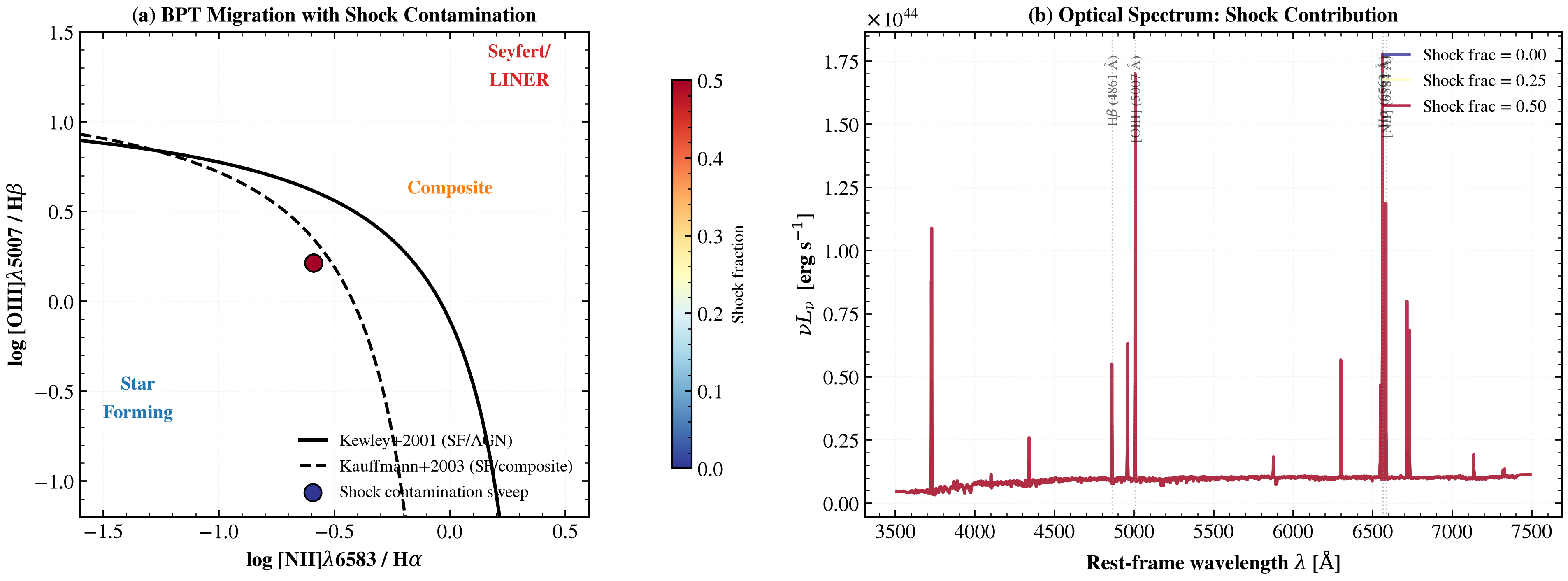
The shock group adds MAPPINGS V shock emission as an additive component to any photoionized nebular backend (Cue, CloudyGrid, CB19, or baked-in). Here we show how increasing shock contamination (shock_frac) moves a star-forming galaxy from the SF locus toward the LI(N)ER/shock region of the BPT diagnostic plane.
Panel 1 sweeps shock_frac from 0 → 0.5 at fixed ionization and metallicity, overlaying Kewley/Kauffmann demarcations. Panel 2 shows the rest-frame optical spectrum at three shock_frac values, revealing how emission lines strengthen when the shock component contributes.
References
import os

os.environ["TF_CPP_MIN_LOG_LEVEL"] = "2"  # suppress XLA/PjRt C++ INFO+WARNING logs

import warnings

import jax
import jax.numpy as jnp
import matplotlib.pyplot as plt
import numpy as np

import tengri
from tengri.plot import setup_style

setup_style()
warnings.filterwarnings("ignore", message=".*BakedInBackend.*")
warnings.filterwarnings("ignore", message=".*deprecated.*")

# --- Load bare-stellar SSP (required for Cue) ---
ssp = tengri.load_ssp("fsps_prsc_miles_chabrier")

# --- BPT demarcation lines ---
log_nii_ha_grid = np.linspace(-1.6, 0.5, 300)

# Kewley+2001 maximum starburst line
log_oiii_hb_kewley = 0.61 / (log_nii_ha_grid - 0.47) + 1.19

# Kauffmann+2003 empirical SF line
log_oiii_hb_kauff = 0.61 / (log_nii_ha_grid - 0.05) + 1.3

# --- Shock fraction sweep on a baseline SF galaxy ---
# Build a star-forming galaxy with fixed photoionized nebular component.
# The shock component is added as an *optional, additive* layer.
model = tengri.SEDModel.build(
    ssp,
    sfh={
        "type": "dpl",
        "all_params": tengri.Fixed(tengri.DEFAULT),
        "alpha": 1.0,
        "beta": 2.5,
        "tau_gyr": 0.1,
        "log_total_mass": 10.0,
    },
    dust_attenuation={
        "law": "power_law",
        "type": "two_component",
        "all_params": tengri.Fixed(tengri.DEFAULT),
        "tau_diff": 0.05,
        "tau_bc": 0.1,
    },
    neb={
        "type": "cue",
        "all_params": tengri.Fixed(tengri.DEFAULT),
        "logU": tengri.Fixed(-2.8),
        "logZ_gas": tengri.Fixed(-0.3),
    },
    # Add the composable shock group: shock_frac will vary, other params fixed.
    shock={
        "type": "mappings",
        "norm": "frac",
        "all_params": tengri.Fixed(tengri.DEFAULT),
        "frac": tengri.Uniform(0.0, 0.5),
        "velocity": tengri.Fixed(300.0),
        "log_density": tengri.Fixed(0.0),
        "b_over_sqrt_n": tengri.Fixed(1.0),
    },
    redshift=tengri.Fixed(0.05),
)

params_base = dict(model.spec.sample(jax.random.PRNGKey(42)))

# --- Compute line ratios across shock_frac sweep ---
shock_fracs = np.linspace(0.0, 0.5, 9)
log_nii_ha_sweep = []
log_oiii_hb_sweep = []

for shock_frac in shock_fracs:
    params = {**params_base, "shock_frac": jnp.float64(shock_frac)}
    lines = model.predict(params).lines

    if lines is not None:
        ha = float(lines.halpha)
        hb = float(lines.hbeta)
        nii = float(lines.nii_6584)
        oiii = float(lines.oiii_5007)

        if ha > 0 and hb > 0 and nii > 0 and oiii > 0:
            log_nii_ha_sweep.append(np.log10(nii / ha))
            log_oiii_hb_sweep.append(np.log10(oiii / hb))
        else:
            # Guard against any unphysical line ratios (e.g., negative fluxes)
            log_nii_ha_sweep.append(np.nan)
            log_oiii_hb_sweep.append(np.nan)
    else:
        log_nii_ha_sweep.append(np.nan)
        log_oiii_hb_sweep.append(np.nan)

log_nii_ha_sweep = np.array(log_nii_ha_sweep)
log_oiii_hb_sweep = np.array(log_oiii_hb_sweep)

# Filter out NaN values for plotting
valid = ~(np.isnan(log_nii_ha_sweep) | np.isnan(log_oiii_hb_sweep))
log_nii_ha_valid = log_nii_ha_sweep[valid]
log_oiii_hb_valid = log_oiii_hb_sweep[valid]
shock_fracs_valid = shock_fracs[valid]

# --- Create figure with two panels ---
fig, (ax1, ax2) = plt.subplots(1, 2, figsize=(13, 5))

# --- Panel 1: BPT diagram with shock_frac sweep ---
# Demarcation lines
mask_k = log_nii_ha_grid < 0.47
ax1.plot(
    log_nii_ha_grid[mask_k],
    log_oiii_hb_kewley[mask_k],
    "k-",
    lw=2.0,
    label="Kewley+2001 (SF/AGN)",
)
mask_kauff = log_nii_ha_grid < 0.05
ax1.plot(
    log_nii_ha_grid[mask_kauff],
    log_oiii_hb_kauff[mask_kauff],
    "k--",
    lw=1.8,
    label="Kauffmann+2003 (SF/composite)",
)

# Region labels
ax1.text(
    -1.35, -0.65, "Star\nForming", fontsize=11, color="#1f77b4", fontweight="bold", ha="center"
)
ax1.text(0.0, 0.6, "Composite", fontsize=11, color="#ff7f0e", fontweight="bold", ha="center")
ax1.text(0.3, 1.2, "Seyfert/\nLINER", fontsize=11, color="#d62728", fontweight="bold", ha="center")

# Shock contamination sweep
if len(shock_fracs_valid) > 0:
    sc = ax1.scatter(
        log_nii_ha_valid,
        log_oiii_hb_valid,
        c=shock_fracs_valid,
        cmap="RdYlBu_r",
        s=100,
        zorder=5,
        edgecolors="black",
        lw=1.0,
        label="Shock contamination sweep",
    )
    cbar = plt.colorbar(sc, ax=ax1, pad=0.12, shrink=0.8)
    cbar.set_label("Shock fraction", fontsize=10)

    # Draw trajectory arrow from low to high shock_frac
    if len(shock_fracs_valid) >= 2:
        ax1.annotate(
            "",
            xy=(log_nii_ha_valid[-1], log_oiii_hb_valid[-1]),
            xytext=(log_nii_ha_valid[0], log_oiii_hb_valid[0]),
            arrowprops=dict(arrowstyle="->", lw=2.0, color="gray", alpha=0.5),
        )

ax1.set_xlabel(r"log [NII]$\lambda$6583 / H$\alpha$", fontsize=12, fontweight="bold")
ax1.set_ylabel(r"log [OIII]$\lambda$5007 / H$\beta$", fontsize=12, fontweight="bold")
ax1.set_xlim(-1.6, 0.6)
ax1.set_ylim(-1.2, 1.5)
ax1.legend(fontsize=10, frameon=False, loc="lower right")
ax1.grid(True, alpha=0.2, linestyle=":")
ax1.set_title("(a) BPT Migration with Shock Contamination", fontsize=12, fontweight="bold")

# --- Panel 2: Optical spectrum at three shock_frac values ---
# Select three representative shock_frac values
selected_fracs = np.array([0.0, 0.25, 0.5])
selected_colors = plt.cm.RdYlBu_r(np.linspace(0, 1, len(selected_fracs)))

# Spectral window: 3500–7500 Å (optical)
wave_min, wave_max = 3500.0, 7500.0

for frac, color in zip(selected_fracs, selected_colors):
    params_spec = {**params_base, "shock_frac": jnp.float64(frac)}
    pred = model.predict(params_spec)

    wave = np.asarray(model.wavelengths)
    sed = np.asarray(pred.rest_sed())

    # Select wavelength range
    mask_wave = (wave >= wave_min) & (wave <= wave_max)

    if np.any(mask_wave):
        wave_spec = wave[mask_wave]
        sed_spec = sed[mask_wave]

        # Convert to nu * L_nu for better visualization
        nu = 2.998e18 / wave_spec
        nu_l_nu = nu * sed_spec

        ax2.plot(
            wave_spec,
            nu_l_nu,
            color=color,
            lw=1.8,
            label=f"Shock frac = {frac:.2f}",
            alpha=0.8,
        )

# Mark major emission lines (rest-frame)
line_markers = {
    r"H$\beta$ (4861 Å)": 4862.68,
    r"[OIII] (5007 Å)": 5008.24,
    r"[NII] (6584 Å)": 6585.28,
    r"H$\alpha$ (6563 Å)": 6564.61,
}

for line_name, line_wave in line_markers.items():
    if wave_min <= line_wave <= wave_max:
        ax2.axvline(line_wave, color="gray", linestyle=":", lw=0.8, alpha=0.5)
        ax2.text(
            line_wave,
            ax2.get_ylim()[1] * 0.95,
            line_name,
            fontsize=8,
            ha="center",
            rotation=90,
            va="top",
            alpha=0.6,
        )

ax2.set_xlabel(r"Rest-frame wavelength $\lambda$ [$\mathrm{\AA}$]", fontsize=12, fontweight="bold")
ax2.set_ylabel(r"$\nu L_\nu$  [erg s$^{-1}$]", fontsize=12, fontweight="bold")
ax2.legend(fontsize=10, frameon=False, loc="upper right")
ax2.grid(True, alpha=0.2, linestyle=":")
ax2.set_title("(b) Optical Spectrum: Shock Contribution", fontsize=12, fontweight="bold")

fig.tight_layout()
plt.savefig("plot_shock_frac_sweep.png", dpi=150, bbox_inches="tight")
Total running time of the script: (0 minutes 2.473 seconds)