Note
Go to the end to download the full example code.
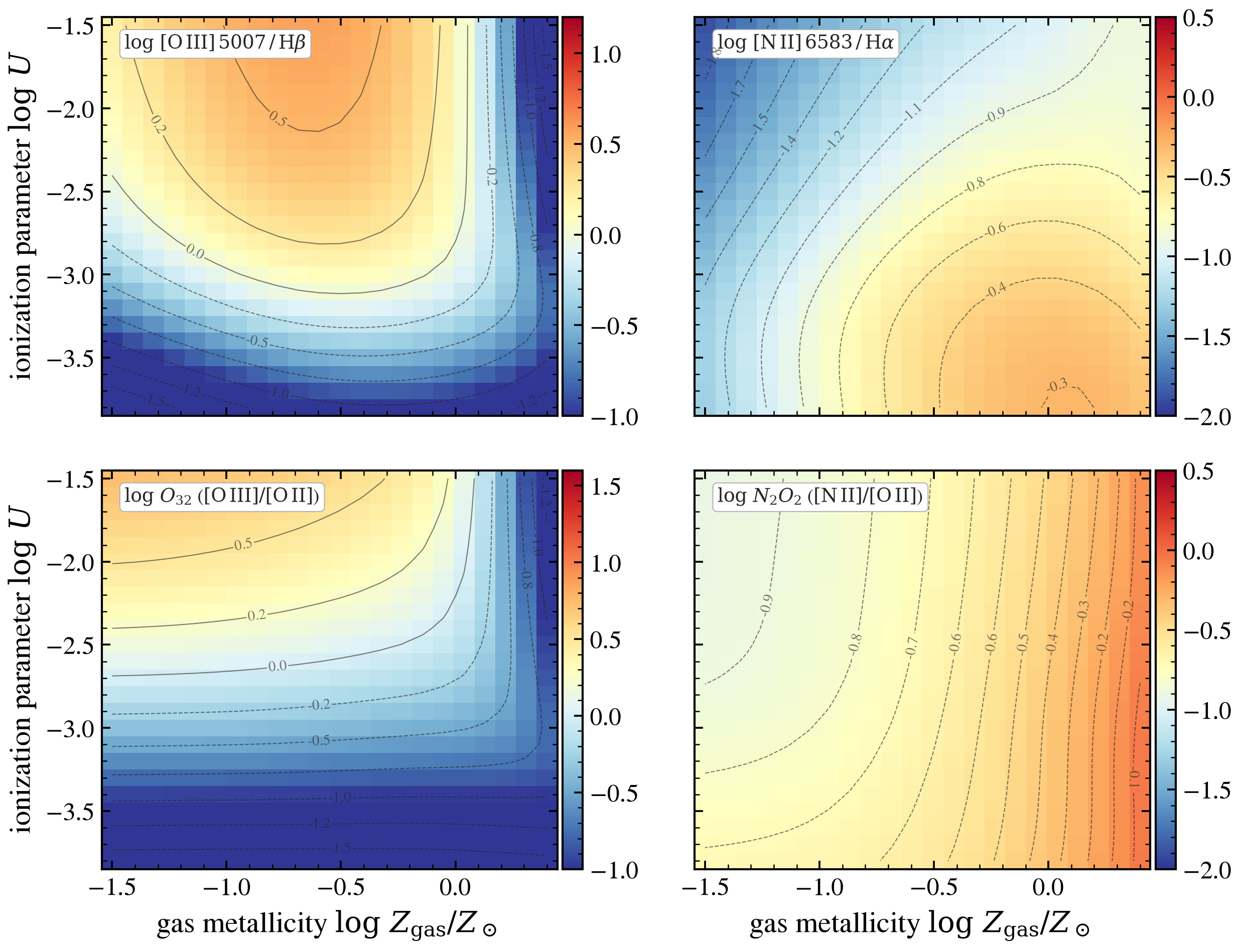
Comprehensive 2D sweep of ionization parameter and metallicity (Cue)
Cue (Li, Leja & Speagle 2023) maps a four-dimensional HII region
control space — ionization parameter log U, gas-phase metallicity
log Z_gas, ionizing-spectrum shape, and dust-to-metal ratio —
onto an emission-line spectrum. A two-dimensional sweep over the two
knobs most users will turn (log U and log Z_gas) is shown for
four diagnostic line ratios.
The grid is built on a young SF galaxy with bare-stellar SSP (Cue requires bare-stellar input — see Cue documentation).
Diagnostics shown (read all from the rest-frame line list):
[O III] 5007 / H_β: ionization-state proxy (BPT y-axis)[N II] 6583 / H_α: N-abundance + ionization (BPT x-axis)[O III] 5007 / [O II] 3727:O32(ionization parameter)[N II] 6583 / [O II] 3727:N2O2(gas metallicity)
The 2D grid subsumes 1D slices: varying logU alone at fixed metallicity (ionization-hardness diagnostic) and varying metallicity alone (abundance evolution). See the heatmap contours for guidance on how the diagnostics respond along each axis.
References:
Li, Leja & Speagle 2023, ApJ, 956, 23 (Cue)
Kewley & Dolphin 2002, ApJ, 549, 716 (logU diagnostics)
Kewley+2019, ARA&A, 57, 511 (modern line-diagnostics review)
import os

os.environ["TF_CPP_MIN_LOG_LEVEL"] = "2"  # suppress XLA/PjRt C++ INFO+WARNING logs

import warnings

import jax
import jax.numpy as jnp
import matplotlib.pyplot as plt
import numpy as np

import tengri
from tengri.plot import setup_style

setup_style()
warnings.filterwarnings("ignore", message=".*BakedInBackend.*")

# Cue knob grid
LOGU_GRID = np.linspace(-3.8, -1.5, 24)
LOGZ_GRID = np.linspace(-1.5, 0.4, 22)

ssp = tengri.load_ssp("fsps_prsc_miles_chabrier")
model = tengri.SEDModel.build(
    ssp,
    sfh={
        "type": "dpl",
        "all_params": tengri.Fixed(tengri.DEFAULT),
        "tau_gyr": 0.3,
        "log_total_mass": 10.0,
        "alpha": 3.0,
        "beta": 2.0,
    },
    dust_attenuation={
        "law": "power_law",
        "type": "two_component",
        "all_params": tengri.Fixed(tengri.DEFAULT),
        "tau_diff": 0.05,
        "tau_bc": 0.1,
    },
    neb={
        "type": "cue",
        "all_params": tengri.Fixed(tengri.DEFAULT),
        "logU": tengri.Uniform(-4.0, -1.0),
        "logZ_gas": tengri.Uniform(-2.0, 0.5),
    },
    redshift=tengri.Fixed(0.05),
)
baseline = dict(model.spec.sample(jax.random.PRNGKey(0)))


SHAPE = (LOGU_GRID.size, LOGZ_GRID.size)
o3_hb = np.empty(SHAPE)
n2_ha = np.empty(SHAPE)
o32 = np.empty(SHAPE)
n2o2 = np.empty(SHAPE)

for i, logu in enumerate(LOGU_GRID):
    for j, logz in enumerate(LOGZ_GRID):
        p = {**baseline, "neb_logU": jnp.float64(logu), "neb_logZ_gas": jnp.float64(logz)}
        lines = model.predict(p).lines
        o3_hb[i, j] = float(lines.oiii_5007 / lines.hbeta)
        n2_ha[i, j] = float(lines.nii_6584 / lines.halpha)
        o32[i, j] = float(lines.oiii_5007 / lines.oii)
        n2o2[i, j] = float(lines.nii_6584 / lines.oii)


def _panel(ax, arr, vmin, vmax, label, n_contours=10):
    """Plot 2D heatmap with contours showing 1D structure."""
    arr = np.where(arr > 0, np.log10(arr), np.nan)
    mesh = ax.pcolormesh(
        LOGZ_GRID, LOGU_GRID, arr, cmap="RdYlBu_r", vmin=vmin, vmax=vmax, shading="auto"
    )
    cs = ax.contour(
        LOGZ_GRID,
        LOGU_GRID,
        arr,
        levels=n_contours,
        colors="0.15",
        linewidths=0.5,
        alpha=0.6,
    )
    ax.clabel(cs, fmt="%.1f", fontsize=7, inline=True, inline_spacing=2)
    ax.text(
        0.05,
        0.92,
        label,
        transform=ax.transAxes,
        fontsize=9,
        color="0.15",
        bbox=dict(boxstyle="round,pad=0.25", fc="white", ec="0.7", lw=0.5),
    )
    return mesh


fig, axes = plt.subplots(2, 2, figsize=(8.6, 6.6), sharex=True, sharey=True)
m1 = _panel(axes[0, 0], o3_hb, -1.0, 1.2, r"$\log\,[\mathrm{O\,III}]\,5007\,/\,\mathrm{H}\beta$")
m2 = _panel(axes[0, 1], n2_ha, -2.0, 0.5, r"$\log\,[\mathrm{N\,II}]\,6583\,/\,\mathrm{H}\alpha$")
m3 = _panel(axes[1, 0], o32, -1.0, 1.6, r"$\log\,O_{32}$ ($[\mathrm{O\,III}]/[\mathrm{O\,II}]$)")
m4 = _panel(
    axes[1, 1], n2o2, -2.0, 0.5, r"$\log\,N_{2}O_{2}$ ($[\mathrm{N\,II}]/[\mathrm{O\,II}]$)"
)

for ax in axes[-1]:
    ax.set_xlabel(r"gas metallicity $\log\,Z_{\rm gas}/Z_\odot$")
for ax in axes[:, 0]:
    ax.set_ylabel(r"ionization parameter $\log\,U$")

for mesh, ax in zip([m1, m2, m3, m4], axes.ravel()):
    fig.colorbar(mesh, ax=ax, pad=0.01)

fig.tight_layout()
plt.savefig("plot_cue_parameter_atlas.png", dpi=150, bbox_inches="tight")
Total running time of the script: (0 minutes 46.992 seconds)