Note
Go to the end to download the full example code.
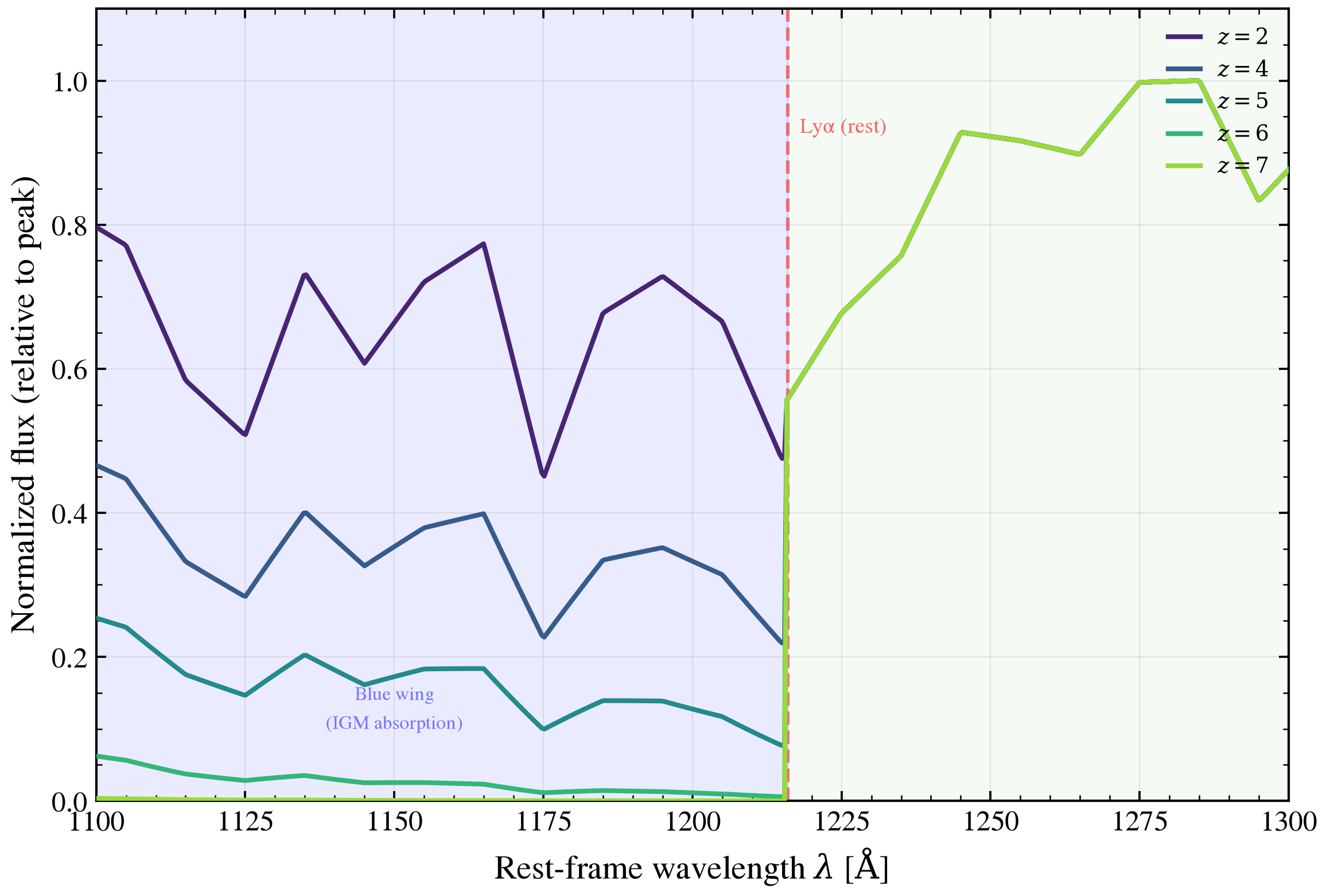
Lyman-alpha profile and IGM blue-wing absorption across redshift
The Lyman-alpha (Lyα) emission line at rest-frame 1216 Å is one of the strongest hydrogen recombination features in star-forming galaxies. As the redshift increases from z = 2 to z = 7, the IGM becomes progressively opaque at wavelengths shortward of Lyα (the “blue wing”), due to cumulative Lyman-series absorption from neutral hydrogen in the intergalactic medium.
a young star-forming galaxy SED with strong Lyα emission, redshifted and IGM-attenuated across five epochs. The characteristic signatures are:
Rest-frame Lyα sits at 1216 Å; in the observer frame it moves to (1+z) × 1216 Å
Wavelengths shortward of Lyα (the Lyman forest) become progressively absorbed at higher redshift due to neutral hydrogen absorption
The red side (Lyα + a few hundred Ångströms) remains mostly unaffected by IGM
At z ≥ 6, the blue wing is severely damped, which is why Lyα emission becomes difficult to detect in high-redshift galaxies
This is the foundational principle behind Lyα-dropout selection and the growing difficulty in detecting Lyα emission at the Epoch of Reionization.
References:
Madau, P. 1995, ApJ, 441, 18 (foundational IGM absorption model)
Inoue, A. T., Iwata, I., Deharveng, J. M., et al. 2014, MNRAS, 442, 1805 (modern IGM prescription used here)
/tengri/src/tengri/forward/orchestrator.py:951: SFHBeforeBigBangWarning: Star formation history forms 100% of its stellar mass before the Big Bang at z=2.00 (cosmic age 3.29 Gyr). That mass is truncated, so the prediction does not reflect the requested SFH: bound the SFH age parameter or the redshift to keep star formation within cosmic time.
  state = component.apply(state, sliced, ssp_data=ssp_data, template_data=template_data)
/tengri/src/tengri/forward/orchestrator.py:951: SFHBeforeBigBangWarning: Star formation history forms 100% of its stellar mass before the Big Bang at z=4.00 (cosmic age 1.54 Gyr). That mass is truncated, so the prediction does not reflect the requested SFH: bound the SFH age parameter or the redshift to keep star formation within cosmic time.
  state = component.apply(state, sliced, ssp_data=ssp_data, template_data=template_data)
/tengri/src/tengri/forward/orchestrator.py:951: SFHBeforeBigBangWarning: Star formation history forms 100% of its stellar mass before the Big Bang at z=5.00 (cosmic age 1.18 Gyr). That mass is truncated, so the prediction does not reflect the requested SFH: bound the SFH age parameter or the redshift to keep star formation within cosmic time.
  state = component.apply(state, sliced, ssp_data=ssp_data, template_data=template_data)
/tengri/src/tengri/forward/orchestrator.py:951: SFHBeforeBigBangWarning: Star formation history forms 100% of its stellar mass before the Big Bang at z=6.00 (cosmic age 0.93 Gyr). That mass is truncated, so the prediction does not reflect the requested SFH: bound the SFH age parameter or the redshift to keep star formation within cosmic time.
  state = component.apply(state, sliced, ssp_data=ssp_data, template_data=template_data)
/tengri/src/tengri/forward/orchestrator.py:951: SFHBeforeBigBangWarning: Star formation history forms 100% of its stellar mass before the Big Bang at z=7.00 (cosmic age 0.76 Gyr). That mass is truncated, so the prediction does not reflect the requested SFH: bound the SFH age parameter or the redshift to keep star formation within cosmic time.
  state = component.apply(state, sliced, ssp_data=ssp_data, template_data=template_data)
import os

os.environ["TF_CPP_MIN_LOG_LEVEL"] = "2"  # suppress XLA/PjRt C++ INFO+WARNING logs

import warnings

import jax
import matplotlib.pyplot as plt
import numpy as np

import tengri
from tengri import igm_transmission
from tengri.plot import setup_style

setup_style()
warnings.filterwarnings("ignore", message=".*BakedInBackend.*")

# Physical constants
C_AA_PER_S = 2.998e18  # Speed of light in Angstrom/second
LYMAN_ALPHA_REST = 1216.0  # Angstrom, rest-frame Lyα wavelength

# Redshifts to display: from local universe to epoch of reionization
REDSHIFTS = [2.0, 4.0, 5.0, 6.0, 7.0]
COLORS = plt.cm.viridis(np.linspace(0.1, 0.85, len(REDSHIFTS)))

# Model configuration: young star-forming galaxy
# Uses the stellar continuum from a young SSP to approximate strong Lyα emission
# (typical in star-forming galaxies at z > 2)
SFH = {
    "type": "dpl",
    "all_params": tengri.Fixed(tengri.DEFAULT),
    "tau_gyr": 0.2,  # Young starburst timescale
    "log_total_mass": 10.0,  # Moderately intense star formation
    "alpha": 3.0,  # Rising SFR at early times
    "beta": 2.0,  # Declining SFR at late times
}

# Minimal dust to preserve continuum strength
DUST = {
    "law": "power_law",
    "type": "two_component",
    "all_params": tengri.Fixed(tengri.DEFAULT),
    "tau_diff": 0.05,
    "tau_bc": 0.05,
}

# Build model with IGM absorption enabled
ssp = tengri.load_ssp()
model = tengri.SEDModel.build(
    ssp,
    sfh=SFH,
    dust_attenuation=DUST,
    igm={"type": "inoue14"},  # Inoue et al. 2014 IGM model
    redshift=tengri.Uniform(1.5, 8.0),
)

# Sample parameters once (redshift will be overridden in the loop)
p_base = dict(model.spec.sample(jax.random.PRNGKey(0)))

# Rest-frame wavelength grid: focused on Lyman-alpha region
wave_rest = np.linspace(1100.0, 1300.0, 512)  # 1100–1300 Å rest-frame

# Create figure
fig, ax = plt.subplots(figsize=(8.0, 5.5))

# Process each redshift
for z, color in zip(REDSHIFTS, COLORS):
    # Override redshift parameter
    params = {**p_base, "redshift": float(z)}

    # Get rest-frame SED
    out = model.predict(params)
    wave_rest_out = np.asarray(model.wavelengths)
    sed_rest = np.asarray(out.rest_sed())

    # Interpolate to our wavelength grid for cleaner visualization
    sed_interp = np.interp(wave_rest, wave_rest_out, sed_rest, left=0, right=0)

    # Transform to observed frame for IGM calculation
    wave_obs = wave_rest * (1.0 + z)

    # Compute IGM transmission in observed frame
    igm_trans = igm_transmission(wave_obs, z_source=z)

    # Apply IGM attenuation in observed frame, then transform flux back
    # Note: IGM operates on F_lambda, and attenuation is wavelength-dependent
    sed_attenuated = sed_interp * igm_trans

    # Normalize for visual clarity (allows comparison of profile shapes)
    i_peak = np.argmax(sed_attenuated)
    sed_norm = sed_attenuated / sed_attenuated[i_peak]

    # Plot rest-frame wavelength vs normalized flux
    ax.plot(
        wave_rest,
        sed_norm,
        color=color,
        lw=2.0,
        label=f"$z = {z:g}$",
        zorder=4,
    )

# Highlight the Lyman-alpha rest-frame position
ax.axvline(LYMAN_ALPHA_REST, color="red", ls="--", lw=1.5, alpha=0.5, zorder=2)
ax.text(
    LYMAN_ALPHA_REST + 2,
    0.95,
    "Lyα (rest)",
    rotation=0,
    fontsize=9,
    color="red",
    alpha=0.6,
    va="top",
)

# Shade the region of blue-wing absorption (shortward of Lyα)
ax.axvspan(1100, LYMAN_ALPHA_REST, alpha=0.08, color="blue", zorder=1)
ax.text(
    1150,
    0.1,
    "Blue wing\n(IGM absorption)",
    fontsize=8,
    ha="center",
    color="blue",
    alpha=0.5,
)

# Shade the red side (mostly unaffected by IGM)
ax.axvspan(LYMAN_ALPHA_REST, 1300, alpha=0.04, color="green", zorder=1)

# Formatting
ax.set(
    xlim=(1100, 1300),
    ylim=(0, 1.1),
    xlabel=r"Rest-frame wavelength $\lambda$ [$\mathrm{\AA}$]",
    ylabel=r"Normalized flux (relative to peak)",
)
ax.legend(frameon=False, fontsize=9, loc="upper right")
ax.grid(True, alpha=0.3, which="major")

fig.tight_layout()
plt.savefig("plot_lyman_alpha_igm_attenuation.png", dpi=150, bbox_inches="tight")