Note
Go to the end to download the full example code.
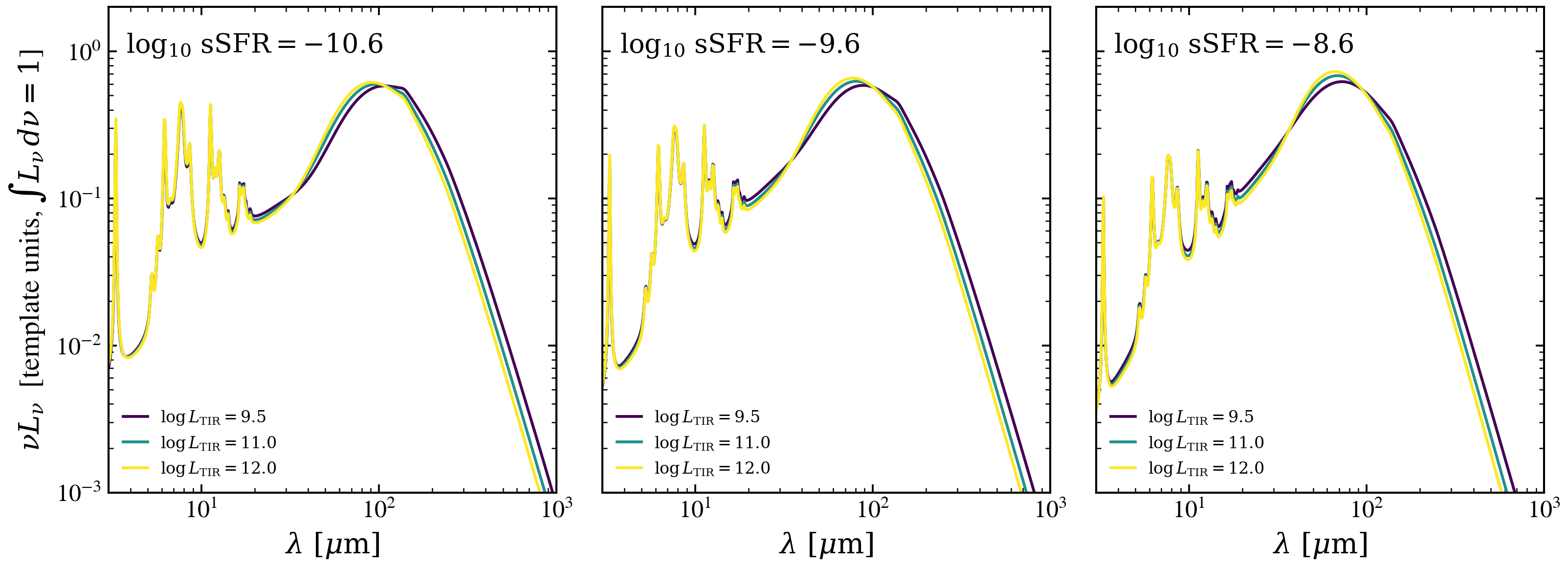
BOSA library: PAH features and FIR peak depend on both sSFR and L_TIR
The BOSA infrared template library is parametrized jointly by total infrared luminosity log L_TIR and specific star formation rate log sSFR. Neither axis alone tells the full story: at fixed sSFR the FIR peak migrates with L_TIR (dust temperature), while at fixed L_TIR the PAH mid-IR forest brightens with sSFR. Three side-by-side panels at fixed sSFR overlay three L_TIR values each, making the 2-D dependence legible in a single figure rather than two skinny 1-D loops.
Reference: BOSA infrared template library (Berta et al. and successors).
import os

os.environ["TF_CPP_MIN_LOG_LEVEL"] = "2"  # suppress XLA/PjRt C++ INFO+WARNING logs

import warnings

import h5py
import matplotlib.pyplot as plt
import numpy as np

from tengri import data_path
from tengri.plot import setup_style

setup_style()
warnings.filterwarnings("ignore", message=".*BakedInBackend.*")
warnings.filterwarnings("ignore", message=".*deprecated.*")

SHOWN_LTIR = (9.5, 11.0, 12.0)
SHOWN_LSSFR = (-10.6, -9.6, -8.6)
C_AA_PER_S = 2.99792458e18

with h5py.File(data_path("bosa_templates.h5"), "r") as f:
    wave_aa = np.asarray(f["wavelength_aa"][:])
    log_ltir = np.asarray(f["log_ltir_grid"][:])
    log_ssfr = np.asarray(f["log_ssfr_grid"][:])
    spectra = np.asarray(f["spectra"][:])

wave_um = wave_aa * 1.0e-4
nu = C_AA_PER_S / wave_aa

fig, axes = plt.subplots(1, 3, figsize=(11.0, 4.2), sharey=True)
cmap = plt.get_cmap("viridis")

for col, lssfr_target in enumerate(SHOWN_LSSFR):
    j = int(np.argmin(np.abs(log_ssfr - lssfr_target)))
    for k, lltir_target in enumerate(SHOWN_LTIR):
        i = int(np.argmin(np.abs(log_ltir - lltir_target)))
        axes[col].plot(
            wave_um,
            nu * spectra[i, j],
            color=cmap(k / (len(SHOWN_LTIR) - 1)),
            lw=1.4,
            label=rf"$\log L_{{\rm TIR}} = {log_ltir[i]:.1f}$",
        )
    axes[col].text(
        0.04,
        0.95,
        rf"$\log_{{10}}\,\mathrm{{sSFR}} = {log_ssfr[j]:+.1f}$",
        transform=axes[col].transAxes,
        va="top",
    )
    axes[col].set(
        xscale="log",
        yscale="log",
        xlim=(3.0, 1.0e3),
        ylim=(1.0e-3, 2.0e0),
        xlabel=r"$\lambda\ [\mu\mathrm{m}]$",
    )
    axes[col].legend(loc="lower left", frameon=False, fontsize=8)

axes[0].set_ylabel(r"$\nu L_\nu$  [template units, $\int L_\nu\, d\nu = 1$]")
fig.tight_layout()
plt.savefig("plot_bosa_grid.png", dpi=150, bbox_inches="tight")