Note
Go to the end to download the full example code.
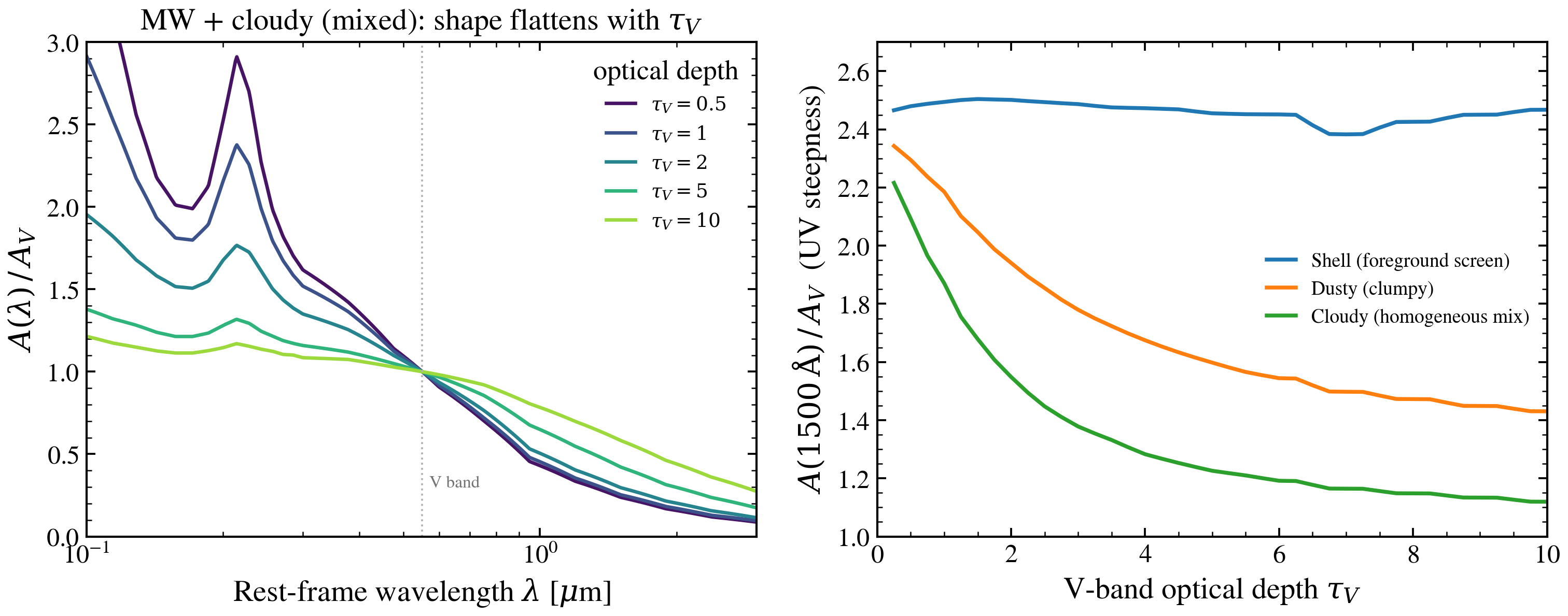
Witt & Gordon 2000: the attenuation shape greys with optical depth
For a foreground dust screen the attenuation curve has a fixed shape — its
amplitude scales with tau_V but the UV-to-optical ratio is constant, so a
single k(lambda) law captures it. Witt & Gordon (2000) showed this breaks
down once dust and stars are mixed: high-tau_V sightlines self-shield, the
short-wavelength photons preferentially escape through low-opacity channels, and
the effective curve greys (flattens) as tau_V rises. The curve shape is
therefore a function of tau_V — which is exactly why tengri ships WG00 as a
radiative-transfer table (FSPS dust_type=3), interpolated in tau_V,
rather than a fixed-shape law.
The left panel overlays the V-normalized curves A(lambda) / A_V for the
homogeneous cloudy (mixed) geometry at five optical depths: the UV bump and
slope visibly flatten as tau_V climbs. The right panel tracks the
far-UV-to-V ratio A(1500 A) / A_V against tau_V for all three WG00
geometries — the shell screen stays flat (fixed shape) while the cloudy and
dusty geometries gray strongly. Everything goes through the public
tengri.dust.wg00_attenuation accessor; no SSP file is required to inspect an
attenuation curve.
References
Witt, A. N. & Gordon, K. D. 2000, ApJ, 528, 799
(“Multiple Scattering in Clumpy Media. II. Galactic Environments”).
Tables as distributed by FSPS (Conroy & Gunn 2010, dust_type=3).
import jax.numpy as jnp
import matplotlib.pyplot as plt
import numpy as np

from tengri.dust import wg00_attenuation
from tengri.plot import setup_style

setup_style()

# Rest-frame grid over the WG00 table validity (0.1-3 um).
wave = jnp.geomspace(1000.0, 30000.0, 500)
wave_um = np.asarray(wave) / 1e4
V = 5500.0  # V band [Angstrom]

TAUS = [0.5, 1.0, 2.0, 5.0, 10.0]
colors = plt.cm.viridis(np.linspace(0.05, 0.85, len(TAUS)))

fig, (ax1, ax2) = plt.subplots(1, 2, figsize=(10.4, 4.3))

# --- Left: V-normalized shape for the mixed (cloudy) geometry ---------------
for tau, c in zip(TAUS, colors):
    a = np.asarray(wg00_attenuation(wave, tau, dust_curve="mw", geometry="cloudy"))
    a_v = float(wg00_attenuation(jnp.array([V]), tau, dust_curve="mw", geometry="cloudy")[0])
    ax1.plot(wave_um, a / a_v, color=c, lw=1.6, label=rf"$\tau_V={tau:g}$")

ax1.axvline(0.55, color="0.7", ls=":", lw=0.9)
ax1.text(0.57, 0.3, "V band", color="0.45", fontsize=8)
ax1.set(
    xscale="log",
    xlabel=r"Rest-frame wavelength $\lambda$ [$\mu$m]",
    ylabel=r"$A(\lambda)\,/\,A_V$",
    title="MW + cloudy (mixed): shape flattens with $\\tau_V$",
    xlim=(0.1, 3.0),
    ylim=(0, 3.0),
)
ax1.legend(frameon=False, fontsize=9, title="optical depth")

# --- Right: far-UV/V graying vs tau_V for the three geometries --------------
taus = np.linspace(0.25, 10.0, 40)
GEOM = [
    ("shell", "Shell (foreground screen)", "#1f77b4"),
    ("dusty", "Dusty (clumpy)", "#ff7f0e"),
    ("cloudy", "Cloudy (homogeneous mix)", "#2ca02c"),
]
for geom, label, color in GEOM:
    ratio = [
        float(wg00_attenuation(jnp.array([1500.0]), t, dust_curve="mw", geometry=geom)[0])
        / float(wg00_attenuation(jnp.array([V]), t, dust_curve="mw", geometry=geom)[0])
        for t in taus
    ]
    ax2.plot(taus, ratio, color=color, lw=1.8, label=label)

ax2.set(
    xlabel=r"V-band optical depth $\tau_V$",
    ylabel=r"$A(1500\,\mathrm{\AA})\,/\,A_V$  (UV steepness)",
    xlim=(0, 10),
    ylim=(1.0, 2.7),
)
ax2.legend(frameon=False, fontsize=9)

plt.tight_layout()
plt.savefig("plot_wg00_tau_v_sweep.png", dpi=150, bbox_inches="tight")