Note
Go to the end to download the full example code.
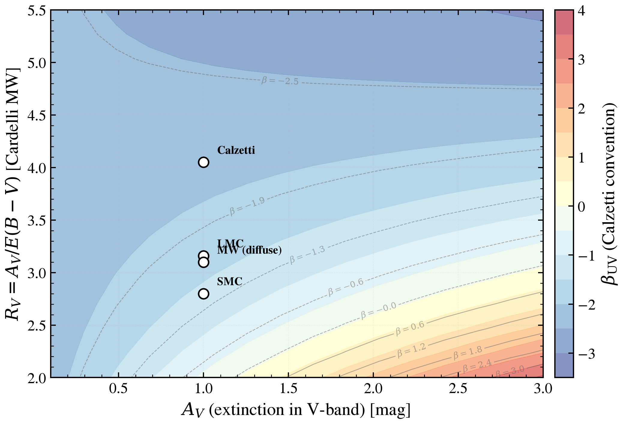
Rv and Av degeneracy in UV slope: the Calzetti trap
At fixed UV slope β_UV (the observable astronomers measure), many (R_V, A_V) pairs produce identical colors — this is a classical dust modeling pitfall. Shows β_UV as contours on the (R_V, A_V) grid for Cardelli MW attenuation. Standard reference points (SMC, LMC, Milky Way diffuse, Calzetti starburst) sit on different iso-β_UV contours, illustrating why dust-law assumptions strongly bias inferred properties.
import warnings

import jax
import matplotlib.pyplot as plt
import numpy as np

import tengri
from tengri.plot import setup_style

setup_style()
warnings.filterwarnings("ignore", message=".*BakedInBackend.*")

# UV slope windows: Calzetti convention (10 wavelength bins, 1268–2580 Å)
WINDOWS = np.array(
    [
        [1268, 1284],
        [1309, 1316],
        [1342, 1371],
        [1407, 1515],
        [1562, 1583],
        [1677, 1740],
        [1760, 1833],
        [1866, 1890],
        [1930, 1950],
        [2400, 2580],
    ]
)
C_AA_PER_S = 2.998e18


def _beta_uv(wave, l_nu):
    """Compute UV slope β_UV in Calzetti convention (fit over 10 windows)."""
    f_lam = l_nu * C_AA_PER_S / wave**2
    mask = np.zeros_like(wave, dtype=bool)
    for lo, hi in WINDOWS:
        mask |= (wave >= lo) & (wave <= hi)
    slope, _ = np.polyfit(np.log10(wave[mask]), np.log10(f_lam[mask]), 1)
    return float(slope)


SFH = {
    "type": "tsnorm",
    "all_params": tengri.Fixed(tengri.DEFAULT),
    "peak_lbt_gyr": 0.05,
    "width_gyr": 0.05,
    "log_total_mass": 8.7,
    "skew": 0.0,
    "trunc": 13.0,
}
ssp = tengri.load_ssp("fsps_prsc_miles_chabrier")


def _model(av, rv):
    return tengri.SEDModel.build(
        ssp,
        sfh=SFH,
        dust_attenuation={
            "type": "two_component",
            "all_params": tengri.Fixed(tengri.DEFAULT),
            "tau_bc": 0.0,
            "tau_diff": av / 1.086,
            # Per-screen pair: this example varies R_V on the diffuse screen,
            # so the two screens deliberately differ and both must be named.
            "law_bc": "power_law",
            "law_diff": "cardelli",
            "Rv": rv,
        },
        redshift=tengri.Fixed(0.05),
    )


av_grid = np.linspace(0.1, 3.0, 16)
rv_grid = np.linspace(2.0, 5.5, 16)
AV_GRID, RV_GRID = np.meshgrid(av_grid, rv_grid)
BETA_GRID = np.zeros_like(AV_GRID)
for i, av in enumerate(av_grid):
    for j, rv in enumerate(rv_grid):
        model = _model(float(av), float(rv))
        p = dict(model.spec.sample(jax.random.PRNGKey(0)))
        out = model.predict(p)
        BETA_GRID[j, i] = _beta_uv(np.asarray(model.wavelengths), np.asarray(out.rest_sed()))
REFS = [(1.0, 2.8, "SMC"), (1.0, 3.16, "LMC"), (1.0, 3.1, "MW (diffuse)"), (1.0, 4.05, "Calzetti")]

fig, ax = plt.subplots(figsize=(7.5, 5.0))

# Contour plot: β_UV iso-lines on (A_V, R_V) grid
levels = np.linspace(BETA_GRID.min(), BETA_GRID.max(), 12)
cs = ax.contour(
    AV_GRID,
    RV_GRID,
    BETA_GRID,
    levels=levels,
    colors="0.4",
    linewidths=0.6,
    alpha=0.5,
)
ax.clabel(cs, inline=True, fontsize=7, fmt=r"$\beta = %.1f$")

# Filled contour as background
cf = ax.contourf(AV_GRID, RV_GRID, BETA_GRID, levels=15, cmap="RdYlBu_r", alpha=0.6)
cbar = fig.colorbar(cf, ax=ax, pad=0.02)
cbar.set_label(r"$\beta_{{\rm UV}}$ (Calzetti convention)")

# Mark standard references
for av, rv, label in REFS:
    ax.plot(
        av,
        rv,
        marker="o",
        markersize=8,
        markerfacecolor="white",
        markeredgecolor="black",
        markeredgewidth=1.2,
        zorder=5,
    )
    ax.text(av + 0.08, rv + 0.08, label, fontsize=9, color="black", fontweight="bold", zorder=5)

ax.set(
    xlabel=r"$A_V$ (extinction in V-band) [mag]",
    ylabel=r"$R_V = A_V / E(B-V)$ [Cardelli MW]",
    xlim=(av_grid.min(), av_grid.max()),
    ylim=(rv_grid.min(), rv_grid.max()),
)
ax.grid(True, alpha=0.2, linestyle=":")

fig.tight_layout()
plt.savefig("plot_rv_av_uv_slope_degeneracy.png", dpi=150, bbox_inches="tight")
Total running time of the script: (0 minutes 5.411 seconds)