Note
Go to the end to download the full example code.
2175 Å bump × UV slope interaction in Kriek & Conroy attenuation
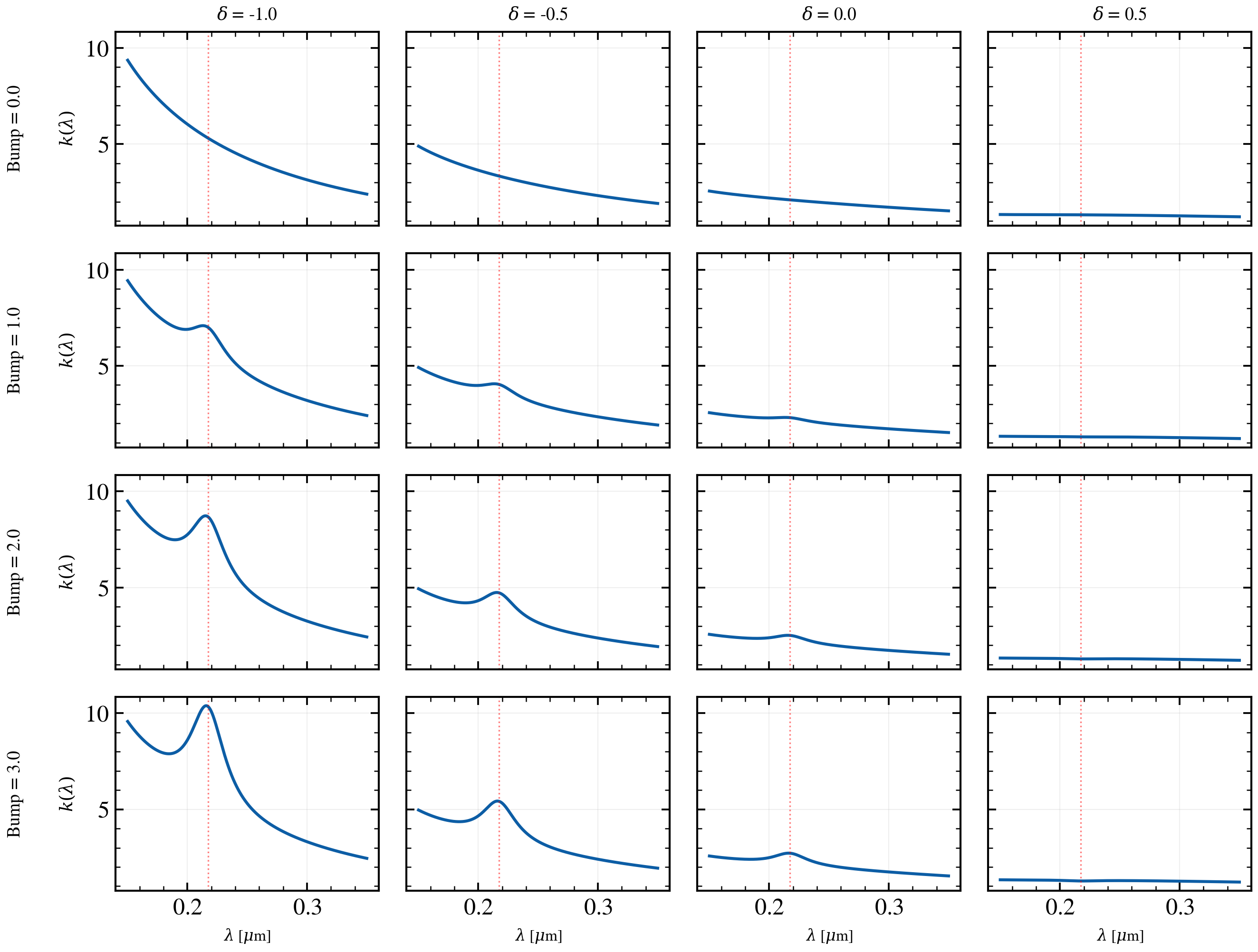
The Kriek & Conroy attenuation law has two degrees of freedom: bump strength and UV slope (δ). Varying both reveals how steeper UV slopes suppress the apparent prominence of the 2175 Å bump relative to the surrounding continuum. We show a 2×2 grid: rows sweep bump strength (0–2 at fixed δ), columns sweep δ slope (−1, +0.5 at fixed bump), revealing the synergy — a steep negative slope (blue wing) enhances bump visibility, while shallow positive slopes (flattened UV) bury the bump in the continuum.
The attenuation curve k(λ) is plotted directly, zoomed on the bump region (1500–3500 Å), to isolate the wavelength-dependent opacity shape.
Reference: Kriek & Conroy 2013, ApJL, 775, L16 (Eq. 5).
import os

os.environ["TF_CPP_MIN_LOG_LEVEL"] = "2"  # suppress XLA/PjRt C++ INFO+WARNING logs

import warnings

import jax.numpy as jnp
import matplotlib.pyplot as plt
import numpy as np

from tengri.dust import resolve_dust_law
from tengri.plot import setup_style

setup_style()
warnings.filterwarnings("ignore", message=".*BakedInBackend.*")

wave = jnp.linspace(1500.0, 3500.0, 1000)
dust_fn = resolve_dust_law("kriek_conroy")

bump_values = np.array([0.0, 1.0, 2.0, 3.0])
delta_values = np.array([-1.0, -0.5, 0.0, 0.5])

fig, axes = plt.subplots(
    len(bump_values), len(delta_values), figsize=(9.0, 7.0), sharex=True, sharey=True
)

for i, bump in enumerate(bump_values):
    for j, delta in enumerate(delta_values):
        ax = axes[i, j]
        k_lambda = dust_fn(wave, dust_bump_strength=bump, dust_delta=delta)
        ax.plot(np.array(wave) / 1e4, np.array(k_lambda), lw=1.5, color="C0")
        ax.axvline(0.2175, ls=":", color="red", lw=0.8, alpha=0.5)
        ax.grid(True, alpha=0.2)

        if i == 0:
            ax.set_title(rf"$\delta$ = {delta:.1f}", fontsize=9)
        if j == 0:
            ax.set_ylabel(r"$k(\lambda)$", fontsize=9)
            ax.text(
                -0.35,
                0.5,
                rf"Bump = {bump:.1f}",
                transform=ax.transAxes,
                rotation=90,
                va="center",
                ha="right",
                fontsize=9,
            )
        if i == len(bump_values) - 1:
            ax.set_xlabel(r"$\lambda$ [$\mu$m]", fontsize=8)

fig.tight_layout()
plt.savefig("plot_bump_delta_joint_grid.png", dpi=150, bbox_inches="tight")