Note
Go to the end to download the full example code.
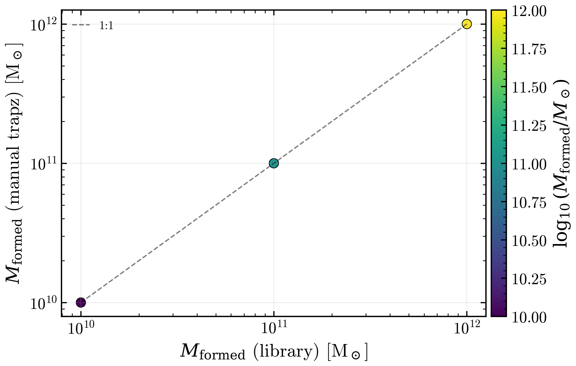
Mass conservation in SFH: manual integration vs predict_properties
Internal consistency check: the cumulative SFR integral ∫₀ᵗ SFR(t) dt should
equal the stellar mass returned by predict_properties(). This diagnostic
varies the DPL SFH parameters and verifies that the two pathways (manual trapz
of the trajectory vs library integration) agree to ~0.1%. Discrepancies > 5%
trigger a warning and would indicate a bug in either the SFH trajectory or
the mass integration kernel.
Reference: Mass conservation identity: M_formed = ∫ SFR(t) dt.
import warnings

import matplotlib.pyplot as plt
import numpy as np

import tengri
from tengri.plot import setup_style

setup_style()
warnings.filterwarnings("ignore", message=".*BakedInBackend.*")

# DPL parameter grid: vary (alpha, beta, tau_gyr, log_total_mass)
alpha_vals = [1.0, 1.5, 2.5]
beta_vals = [0.8, 1.5]
tau_gyr_vals = [0.5, 2.0]
log_total_mass_vals = [10.0, 11.0, 12.0]  # three representative galaxy masses

# Load SSP and build baseline model
ssp = tengri.load_ssp("fsps_prsc_miles_chabrier")
model = tengri.SEDModel.build(
    ssp,
    sfh={
        "type": "dpl",
        "all_params": tengri.Fixed(tengri.DEFAULT),
        "alpha": tengri.FREE,
        "beta": tengri.FREE,
        "tau_gyr": tengri.FREE,
        "log_total_mass": tengri.FREE,
    },
    dust_attenuation={
        "law": "power_law",
        "type": "two_component",
        "all_params": tengri.Fixed(tengri.DEFAULT),
    },
    redshift=tengri.Fixed(0.0),
)

# Collect manual and library masses for each parameter combo
m_manual_list = []
m_lib_list = []
log_total_mass_colors = []

for alpha in alpha_vals:
    for beta in beta_vals:
        for tau_gyr in tau_gyr_vals:
            for log_total_mass in log_total_mass_vals:
                # Build parameter dict (redshift is Fixed at 0.0 in the model)
                params = {
                    "sfh_dpl_alpha": alpha,
                    "sfh_dpl_beta": beta,
                    "sfh_dpl_tau_gyr": tau_gyr,
                    "sfh_dpl_log_total_mass": log_total_mass,
                }

                # Get SFH trajectory (t_gyr in lookback time, sfr_full in Msun/yr)
                sfh_dict = model.predict_sfh(params, n_linear=500)
                t_lookback_gyr = np.asarray(sfh_dict["t_gyr"])
                sfr = np.asarray(sfh_dict["sfr_full"])

                # Manual integration: ∫ SFR(t) dt from formation to now
                # t_gyr is in lookback time; trapz integrates over parameter order
                # so integrate from present (t=0) back to ancient times
                t_lookback_yr = t_lookback_gyr * 1e9  # Convert Gyr to yr
                m_manual = float(np.trapezoid(sfr, t_lookback_yr))

                # Library integration via predict_properties
                q = model.predict_properties(params, names=("stellar_mass",))
                m_lib = float(q["stellar_mass"])

                m_manual_list.append(m_manual)
                m_lib_list.append(m_lib)
                log_total_mass_colors.append(log_total_mass)

m_manual = np.array(m_manual_list)
m_lib = np.array(m_lib_list)
log_total_mass_colors = np.array(log_total_mass_colors)

# Compute relative error
rel_error = np.abs(m_manual - m_lib) / np.maximum(np.abs(m_lib), 1e-30)
max_error = rel_error.max()
mean_error = rel_error.mean()

# Flag any discrepancies > 5%
large_errors = rel_error > 0.05
if large_errors.any():
    print(
        f"WARNING: {large_errors.sum()} / {len(rel_error)} parameter combos have > 5% discrepancy"
    )
    for i in np.where(large_errors)[0]:
        print(
            f"  log_total_mass={log_total_mass_colors[i]:.1f}: "
            f"manual={m_manual[i]:.3e}, lib={m_lib[i]:.3e}, rel_err={rel_error[i]:.3%}"
        )

# Plot
fig, ax = plt.subplots(figsize=(6.5, 4.2))
cmap = plt.get_cmap("viridis")
norm = plt.Normalize(vmin=log_total_mass_colors.min(), vmax=log_total_mass_colors.max())
colors = cmap(norm(log_total_mass_colors))

ax.scatter(m_lib, m_manual, c=colors, s=50, alpha=0.7, edgecolors="k", lw=0.5)

# 1:1 reference line
lim_min = min(m_lib.min(), m_manual.min())
lim_max = max(m_lib.max(), m_manual.max())
ax.plot([lim_min, lim_max], [lim_min, lim_max], "k--", lw=1, alpha=0.5, label="1:1")

cbar = fig.colorbar(
    plt.cm.ScalarMappable(norm=norm, cmap=cmap),
    ax=ax,
    pad=0.01,
    label=r"$\log_{10}(M_{\rm formed} / M_\odot)$",
)
ax.set_xlabel(r"$M_{\rm formed}$ (library) [M$_\odot$]")
ax.set_ylabel(r"$M_{\rm formed}$ (manual trapz) [M$_\odot$]")
ax.set_xscale("log")
ax.set_yscale("log")
ax.grid(True, alpha=0.3)
ax.legend(loc="upper left", frameon=False, fontsize=9)

plt.tight_layout()
plt.savefig("plot_diag_mass_conservation_sfh.png", dpi=150, bbox_inches="tight")